Interpolation of electron-phonon matrix elements
Note
Hands-on based on QE-v7.3 and EPW-v5.8
In this session we will learn to use the core capabilities of EPW.
In particular, we will focus on how to check the quality of Wannier
interpolation of physical quantities for a future production run.
You are advised to run the calculations in your scratch directory and
follow the instructions carefully. Unless you are an experienced user of
EPW and Quantum ESPRESSO, do not change the directory structure
and the parameters in jobscript. You can start by creating the working
directory in your scratch folder and copying the tar file which contains
all necessary files for this tutorial and extracting it. Then, go to the
directory of the first exercise:
$ cd $SCRATCH
$ cp /work2/05193/sabyadk/stampede3/EPWSchool2024/tutorials/Tue.6.Lafuente.tar .
$ tar -xvf Tue.6.Lafuente.tar ; cd Tue.6.Lafuente/exercise1
Exercise 1: Metallic Pb
In this exercise we will calculate physical properties of metallic Pb
using Quantum ESPRESSO and repeat the same calculations through
Wannier interpolation using EPW. We will then compare them to check
the interpolation quality. After assessing interpolation quality, we
will calculate the phonon linewidth for Pb.
1st step: Run a self-consistent calculation on a homogeneous \(8 \times 8 \times 8\) k-point grid and a phonon calculation on a homogeneous \(3 \times 3 \times 3\) q-point grid using the following inputs and jobscript:
Note: The energy cutoff ecutwfc needed for convergence should be 90 Ry.
$ cd phonon
$ sbatch job.ph
job.ph
#!/bin/bash
#SBATCH -J myjob              # Job name
#SBATCH -N 1                  # Total # of nodes
#SBATCH --ntasks-per-node 24
#SBATCH -t 01:00:00           # Run time (hh:mm:ss)
#SBATCH -A DMR23030
#SBATCH -p skx
#SBATCH --reservation=NSF_Summer_School_Tue

module list

# Launch MPI code...
export PATHQE=/work2/05193/sabyadk/stampede3/EPWSchool2024/q-e

ibrun $PATHQE/bin/pw.x -nk 4 -in scf.in > scf.out
ibrun $PATHQE/bin/ph.x -nk 4 -in ph.in > ph.out
--                                                                                        scf.in
 &control
    calculation='scf'
    restart_mode='from_scratch',
    prefix='pb',
    pseudo_dir = '../',
    outdir='./'
 /
 &system
    ibrav=  2,
    celldm(1) = 9.2225583816,
    nat= 1,
    ntyp= 1,
    ecutwfc = 30.0
    occupations='smearing',
    smearing='marzari-vanderbilt',
    degauss=0.05
 /
 &electrons
    conv_thr =  1.0d-10
    mixing_beta = 0.7
 /
ATOMIC_SPECIES
 Pb 207.2 pb_s.UPF
ATOMIC_POSITIONS
 Pb 0.00 0.00 0.00
K_POINTS {automatic}
 8 8 8 0 0 0
--                                                                                        ph.in
&inputph
prefix = 'pb',
fildyn = 'pb.dyn.xml',
fildvscf = 'dvscf',
ldisp = .true.,
nq1 = 3,
nq2 = 3,
nq3 = 3,
tr2_ph = 1.0d-16
/
ph.in tells the code to write on file the
change of the self-consistent potential due to phonon perturbations,
\(\partial_{\mathbf{q}\nu}V^{\rm scf}\), that is needed to compute the
electron-phonon matrix elements.ph.out, locate the list of 4 irreducible
\(\mathbf{q}\) points in the Brillouin Zone (IBZ):Dynamical matrices for ( 3, 3, 3) uniform grid of q-points
( 4 q-points):
N xq(1) xq(2) xq(3)
1 0.000000000 0.000000000 0.000000000
2 -0.333333333 0.333333333 -0.333333333
3 0.000000000 0.666666667 0.000000000
4 0.666666667 -0.000000000 0.666666667
pb.dyn0 file. If you type ls, you can see pb.dynX.xml file
containing the dynamical matrix has been produced for each irreducible
\(\mathbf{q}\) point. The dvscf files are all named pb.dvscf1 and are
located inside the _ph0/pb.q_X/ folders, except for the one
corresponding to the first \(\mathbf{q}\) point (\(\Gamma\)) that is
located in _ph0/..xml
format, which is advisable, because we specified it in the ph.in
input with fildyn = ’pb.dyn.xml’.q2r.x:$ /work2/05193/sabyadk/stampede3/EPWSchool2024/q-e/bin/q2r.x -in q2r.in > q2r.out
--                                                                                        q2r.in
&input
zasr='simple', fildyn='pb.dyn.xml', flfrc='pb333.fc'
/
Note in the output if the Fast Fourier transform (FFT) was successful:
fft-check success (sum of imaginary terms < 10^-12)
pb333.fc.xml).matdyn.x:$ /work2/05193/sabyadk/stampede3/EPWSchool2024/q-e/bin/matdyn.x -in matdyn.in > matdyn.out
--                                                                                     matdyn.in
&input
  asr              = 'simple',
  flfrc            = 'pb333.fc.xml'
  flfrq            = 'pb.freq'
  q_in_band_form   = .true.
  q_in_cryst_coord = .true.
/
  6
  0.000 0.000 0.000  30 ! \Gamma
  0.500 0.000 0.500  30 ! X
  0.500 0.250 0.750  30 ! W
  0.500 0.500 0.500  30 ! L
  0.000 0.000 0.000  30 ! \Gamma
  0.375 0.375 0.750  30 ! K
This produces the file named pb.freq.gp with the phonon frequencies
along the path, expressed in cm\(^{-1}\) unit. This will be
checked against the phonon frequencies along the same path from EPW.
3rd step: Gather the .dyn and .dvscf files into a new save/
directory which EPW will read. The files in _ph0/pb.phsave/
containing the displacement patterns are also needed. This can be done
using the pp.py python script which is included in the EPW/bin
distribution:
$ python3 /work2/05193/sabyadk/stampede3/EPWSchool2024/q-e/EPW/bin/pp.py
prefix of your calculation
(pb):Enter the prefix used for PH calculations (e.g. diam)
pb
numpy on your desktop. Just type
“pip install numpy” and run the script again.python3 $PATHQE/EPW/bin/pp.py << EOF
pb
EOF
4th step: Run a non self-consistent calculation for electronic band structures using the charge density and other outputs from the previous self-consistent run:
$ cd ../band
$ sbatch job.band
--                                                                                      job.band
#!/bin/bash
#SBATCH -J myjob              # Job name
#SBATCH -N 1                  # Total # of nodes
#SBATCH --ntasks-per-node 8
#SBATCH -t 01:00:00           # Run time (hh:mm:ss)
#SBATCH -A DMR23030
#SBATCH -p skx
#SBATCH --reservation=NSF_Summer_School_Tue

module list

# Launch MPI code...
export PATHQE=/work2/05193/sabyadk/stampede3/EPWSchool2024/q-e

mkdir pb.save
cp ../phonon/pb.save/charge-density.dat pb.save/
cp ../phonon/pb.save/data-file-schema.xml pb.save/

ibrun $PATHQE/bin/pw.x -nk 4 -in nscf.in > nscf.out
--                                                                                       nscf.in
 &control
    calculation='bands'
    restart_mode='from_scratch',
    prefix='pb',
    pseudo_dir = '../',
    outdir='./'
 /
 &system
    ibrav=  2,
    celldm(1) = 9.2225583816,
    nat= 1,
    ntyp= 1,
    ecutwfc = 30.0
    occupations='smearing',
    smearing='marzari-vanderbilt',
    degauss=0.05
    nbnd=10
 /
 &electrons
    conv_thr =  1.0d-10
    mixing_beta = 0.7
 /
ATOMIC_SPECIES
 Pb 207.2 pb_s.UPF
ATOMIC_POSITIONS
 Pb 0.00 0.00 0.00
K_POINTS crystal_b
  6
  0.000 0.000 0.000  30 ! \Gamma
  0.500 0.000 0.500  30 ! X
  0.500 0.250 0.750  30 ! W
  0.500 0.500 0.500  30 ! L
  0.000 0.000 0.000  30 ! \Gamma
  0.375 0.375 0.750  30 ! K
calculation=’bands’ and
calculation=’nscf’ is that the former uses exclusively the
k-point provided while the latter might add points to respect
crystal symmetry.Then, run the program of bands.x to obtain the band structure data:
$ /work2/05193/sabyadk/stampede3/EPWSchool2024/q-e/bin/bands.x -in bands.in > bands.out
--                                                                                      bands.in
&BANDS
  prefix = 'pb'
  lsym   = .false.
/
This will produce the file named bands.out.gnu which will be
compared with the interpolated electronic band structure from EPW.
5th step: Run a non self-consistent calculation on a homogeneous
\(6\times6\times6\) \(\mathbf{k}\)-point grid for generating the input
of wave functions for EPW and an EPW calculation for the Wannier
interpolation of electronic band structure and phonon dispersion along
the high-symmetry lines:
$ cd ../epw1
$ sbatch job.epw1
--                                                                                      job.epw1
#!/bin/bash
#SBATCH -J myjob              # Job name
#SBATCH -N 1                  # Total # of nodes
#SBATCH --ntasks-per-node 8
#SBATCH -t 01:00:00           # Run time (hh:mm:ss)
#SBATCH -A DMR23030
#SBATCH -p skx
##SBATCH --reservation=NSF_Summer_School_Tue

module list

# Launch MPI code...
export PATHQE=/work2/05193/sabyadk/stampede3/EPWSchool2024/q-e

mkdir pb.save
cp ../phonon/pb.save/charge-density.dat pb.save/
cp ../phonon/pb.save/data-file-schema.xml pb.save/

ibrun $PATHQE/bin/pw.x -nk 4 -in nscf.in > nscf.out
ibrun $PATHQE/bin/epw.x -nk 8 -in epw1.in > epw1.out
--                                                                                       nscf.in
 &control
    calculation='nscf'
    restart_mode='from_scratch',
    prefix='pb',
    pseudo_dir = '../',
    outdir='./'
 /
 &system
    ibrav=  2,
    celldm(1) = 9.2225583816,
    nat= 1,
    ntyp= 1,
    ecutwfc = 30.0
    occupations='smearing',
    smearing='marzari-vanderbilt',
    degauss=0.05
    nbnd=10
 /
 &electrons
    conv_thr =  1.0d-10
    mixing_beta = 0.7
 /
ATOMIC_SPECIES
 Pb 207.2 pb_s.UPF
ATOMIC_POSITIONS
 Pb 0.00 0.00 0.00
K_POINTS crystal
216
  0.00000000  0.00000000  0.00000000  4.629630e-03
  0.00000000  0.00000000  0.16666667  4.629630e-03
...
--                                                                                       epw1.in
&inputepw
  prefix      = 'pb',
  amass(1)    = 207.2
  outdir      = './'
  dvscf_dir   = '../phonon/save'

  etf_mem     = 0

  elph        = .true.
  epbwrite    = .true.
  epbread     = .false
  epwwrite    = .true.
  epwread     = .false.

  wannierize  = .true.
  nbndsub     =  4
  bands_skipped = 'exclude_bands = 1-5'
  num_iter    = 300
  dis_win_max = 21
  dis_froz_max= 13.5
  proj(1)     = 'Pb:sp3'
  wannier_plot= .true.
  wdata(1)    = 'bands_plot = .true.'
  wdata(2)    = 'begin kpoint_path'
  wdata(3)    = 'G 0.00 0.00 0.00 X 0.00 0.50 0.50'
  wdata(4)    = 'X 0.00 0.50 0.50 W 0.25 0.50 0.75'
  wdata(5)    = 'W 0.25 0.50 0.75 L 0.50 0.50 0.50'
  wdata(6)    = 'L 0.50 0.50 0.50 G 0.00 0.00 0.00'
  wdata(7)    = 'G 0.00 0.00 0.00 K 0.375 0.375 0.75'
  wdata(8)    = 'end kpoint_path'
  wdata(9)    = 'bands_num_points = 10'
  wdata(10)   = 'dis_num_iter      = 200'
  wdata(11)   = 'num_print_cycles  = 10'
  wdata(12)   = 'conv_tol = 1E-12'
  wdata(13)   = 'conv_window = 4'

  nkf1         = 1
  nkf2         = 1
  nkf3         = 1
  nqf1         = 1
  nqf2         = 1
  nqf3         = 1

  nk1         = 6
  nk2         = 6
  nk3         = 6
  nq1         = 3
  nq2         = 3
  nq3         = 3
 /
Note 1: In some cases, pw.x calculates additional k-points
which are not provided in the k-point list of the input. If this
happens, you need to use the keyword of calculation=’bands’ instead
of calculation=’nscf’. Also note that the k and q grids need
to be commensurate, with the k grid at least of the size of the
q grid. Since we chose a \(6\times6 \times6\) k-point grid,
the \(3\times 3 \times3\) k-point grid used in the phonon
calculation is appropriate, however a \(6\times6 \times6\)
q-point grid would be needed in order to interpolate more accurately
the dynamical matrix and the electron-phonon matrix elements. For
computational efficiency (see Phys. Rev. Research 3, 043022
(2021)),
we recommend using the same k-point and q grids.
dvscf_dir = ’../phonon/save’ we specify the
directory where the .dyn, .dvscf and patterns files are stored.EPW will perform a Wannierzation, unfolding of
the matrix elements from the IBZ on full BZ coarse grids, and Fourier
transformation of the quantities into real space.Wannierization using
Wannier90as a library. In the output ofepw1.outyou can find the Wannier function centers and spreads obtained:Wannier Function centers (cartesian, alat) and spreads (ang): ( 0.07779 0.07779 0.07779) : 2.22274 ( 0.07779 -0.07779 -0.07779) : 2.22274 ( -0.07779 0.07779 -0.07779) : 2.22274 ( -0.07779 -0.07779 0.07779) : 2.22274
while the full output from the
Wannier90run is in the file ofpb.wout. The input keywords for the Wannierization are in the block followingwannierize = .true..nbndsubcorresponds to the number of Wannier functions (4, starting from Pb sp\(^3\) orbitals as the initial guess), whilebands_skipped = ...specifies the list of bands not wannierized (generally a set of bands lying at lower energies, such as semicore states in this example). For the other input keywords you can refer to the page at https://docs.epw-code.org/doc/Inputs.html. It is also possible to add extra keywords that are read by Wannier90 by using the input keyword ofwdata(index)with increasing index number. Here we are askingWannier90to plot the electronic band structure and we specify high symmetry points for this. As a result, the code will produce the following filespb_band.dat,pb_band.gnu, andpb_band.kpt.In addition, with the input keyword of
wannier plot= .true.we can generate directly and efficiently inEPWthe cube files containing real-space Wannier functions which can be plotted by using the plotting softwares such asVMDandVESTA; the plot ofpb_00001.cubeWannier function should look like this: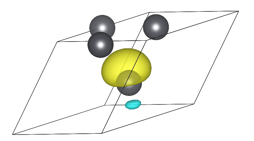
Calculate the electron-phonon matrix elements on the (k, k + q) points for each irreducible q-point in the Brillouin zone and unfold to the full Brillouin zone using symmetries. This is the most expensive part of the run. In the output you can see:
     ===================================================================
     irreducible q point #    1
     ===================================================================

     Symmetries of small group of q: 48
          in addition sym. q -> -q+G:

     Number of q in the star =    1
     List of q in the star:
          1   0.000000000   0.000000000   0.000000000
     Imposing acoustic sum rule on the dynamical matrix

        q(    1 ) = (   0.0000000   0.0000000   0.0000000 )
...
Transform all quantities from reciprocal (Bloch) space to real (Wannier) space and store on file the resulting matrices and additional information needed for restarting a calculation (
pb.epmatwp,crystal.fmt,vmedata.fmt,wigner.fmt, andepwdata.fmtfiles):Writing Hamiltonian, Dynamical matrix and EP vertex in Wann rep to file
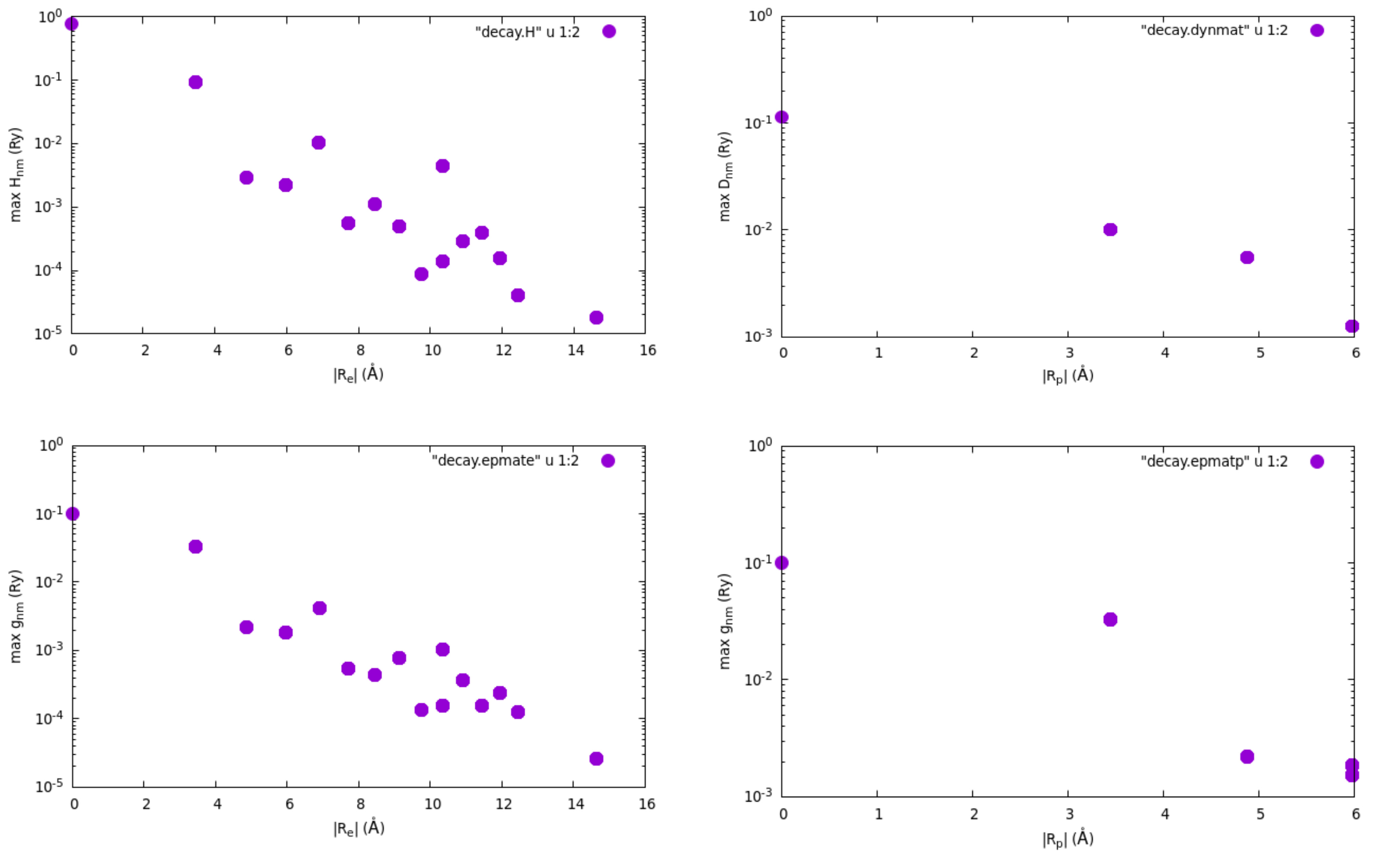
Finally, the Wannier-Fourier interpolation technique is based on the
decay properties of the Wannier functions and of the phonon perturbation
in real space. To check how each quantity is decaying within the
supercell corresponding to our initial k and q grids, we can
plot the files of decay.H (Hamiltonian), decay.dynmat (dynamical
matrix) and decay.epmate (decay.epmatp) (electron-phonon matrix
elements). You can obtain the following plots (note the log scale on the
y axis) using gnuplot and assuming that you are connected with X11
support on Frontera and you are in the epw folder:
$ gnuplot
gnuplot> set encoding iso_8859_1
gnuplot> set logscale y
gnuplot> set format y "10^{%L}"
gnuplot> set pointsize 2
gnuplot> set xlabel "|R_e| (\305)"
gnuplot> set ylabel "max H_{nm} (Ry)"
gnuplot> plot "decay.H" u 1:2 w p pt 7
gnuplot> set xlabel "|R_p| (\305)"
gnuplot> set ylabel "max D_{nm} (Ry)"
gnuplot> plot "decay.dynmat" u 1:2 w p pt 7
gnuplot> set xlabel "|R_e| (\305)"
gnuplot> set ylabel "max g_{nm} (Ry)"
gnuplot> plot "decay.epmate" u 1:2 w p pt 7
gnuplot> set xlabel "|R_p| (\305)"
gnuplot> set ylabel "max g_{nm} (Ry)"
gnuplot> plot "decay.epmatp" u 1:2 w p pt 7
gnuplot> exit
pb_band.kpt file produced by Wannier90 to specify
that the points are in crystal units:43 crystal pb_band.kpt
0.000000 0.000000 0.000000 1.0
0.000000 0.050000 0.050000 1.0
0.000000 0.100000 0.100000 1.0
0.000000 0.150000 0.150000 1.0
0.000000 0.200000 0.200000 1.0
0.000000 0.250000 0.250000 1.0
0.000000 0.300000 0.300000 1.0
0.000000 0.350000 0.350000 1.0
...
Then move to the second folder for the restart calculation:
$ cd ../epw2
$ ln -s ../epw1/pb.epmatwp .
$ ln -s ../epw1/pb.ukk .
$ ln -s ../epw1/*.fmt .
$ ln -s ../epw1/pb_band.kpt .
$ sbatch job.epw2
#!/bin/bash                                                                            job.epw2
#!/bin/bash
#SBATCH -J myjob              # Job name
#SBATCH -N 1                  # Total # of nodes
#SBATCH --ntasks-per-node 8
#SBATCH -t 01:00:00           # Run time (hh:mm:ss)
#SBATCH -A DMR23030
#SBATCH -p skx
##SBATCH --reservation=NSF_Summer_School_Tue

module list

# Launch MPI code...
export PATHQE=/work2/05193/sabyadk/stampede3/EPWSchool2024/q-e

ibrun $PATHQE/bin/epw.x -nk 8 -in epw2.in > epw2.out
ibrun $PATHQE/bin/epw.x -nk 8 -in epw3.in > epw3.out
--                                                                                      epw2.in
&inputepw
  prefix      = 'pb',
  amass(1)    = 207.2
  outdir      = './'
  dvscf_dir   = '../phonon/save'

  etf_mem     = 0

  elph        = .true.
  epbwrite    = .false.
  epbread     = .false
  epwwrite    = .false.
  epwread     = .true.

  wannierize  = .false.
  nbndsub     =  4
  bands_skipped = 'exclude_bands = 1-5'
  num_iter    = 300
  dis_win_max = 21
  dis_froz_max= 13.5
  proj(1)     = 'Pb:sp3'

  band_plot   = .true.
  fsthick     = 100    ! eV - should be large here for bandstructure plot

  filkf       = 'pb_band.kpt'
  filqf       = 'pb_band.kpt'

  nk1         = 6
  nk2         = 6
  nk3         = 6
  nq1         = 3
  nq2         = 3
  nq3         = 3
 /
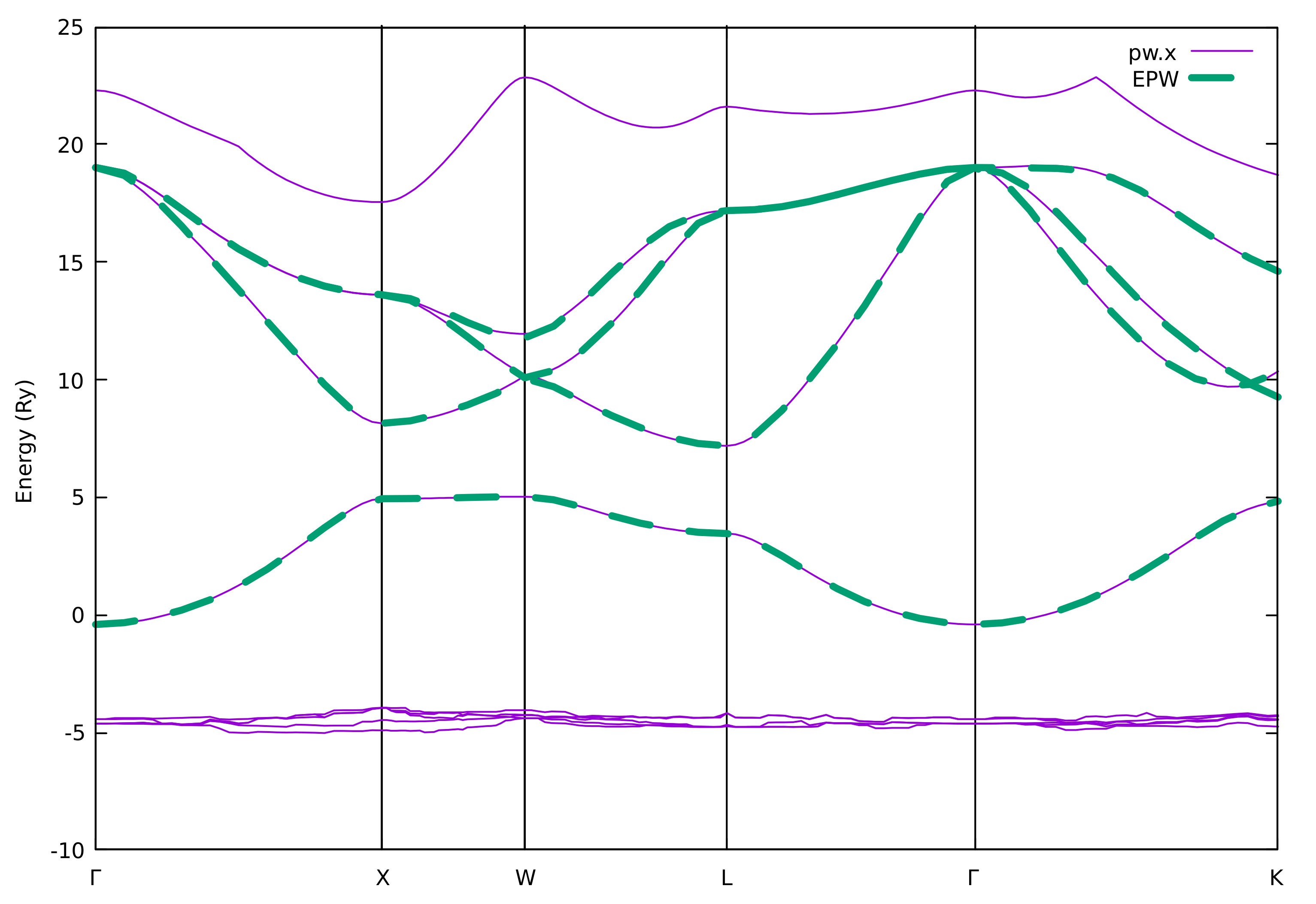
We should always check whether the Wannier-interpolated electron and
phonon band structures match well to those calculated using pw.x and
matdyn.x, respectively. With the input flag of
band_plot = .true. in epw2.in we instructed EPW to save on
files the interpolated electronic bands (band.eig) and phonon
frequencies (phband.freq) and we chose to interpolate them onto the
same Brillouin-zone path as previous pw.x and matdyn.x runs.
This path is read from the file produced by wannier90 in the
previous run and called pb_band.kpt, which is specified by the
keywords of filkf and filqf. To extract easily the data to plot,
you can run the plotband.x program from the Quantum ESPRESSO
package and enter the input file (band.eig or phband.freq), the
energy range (for example, -1 20), the output file with the data to plot
(band.dat or freq.dat). The other inputs are not relevant and
simply push the ENTER key when asked:
$ /work2/05193/sabyadk/stampede3/EPWSchool2024/q-e/bin/plotband.x
     Input file > band.eig
Reading    4 bands at     43 k-points
Range:   -0.4085   19.0142eV  Emin, Emax, [firstk, lastk] > -1 20
high-symmetry point:  0.0000 0.0000 0.0000   x coordinate   0.0000
high-symmetry point:  0.0000 1.0000 0.0000   x coordinate   1.0000
high-symmetry point: -0.5000 1.0000 0.0000   x coordinate   1.5000
high-symmetry point: -0.5000 0.5000 0.5000   x coordinate   2.2071
high-symmetry point:  0.0000 0.0000 0.0000   x coordinate   3.0731
high-symmetry point: -0.7500 0.7500 0.0000   x coordinate   4.1338
output file (gnuplot/xmgr) > band.dat
bands in gnuplot/xmgr format written to file band.dat
output file (ps) >
stopping ...

$ /work2/05193/sabyadk/stampede3/EPWSchool2024/q-e/bin/plotband.x
     Input file > phband.freq
Reading    3 bands at     43 k-points
Range:    0.0000   13.9958eV  Emin, Emax, [firstk, lastk] > 0 14
high-symmetry point:  0.0000 0.0000 0.0000   x coordinate   0.0000
high-symmetry point:  0.0000 1.0000 0.0000   x coordinate   1.0000
high-symmetry point: -0.5000 1.0000 0.0000   x coordinate   1.5000
high-symmetry point: -0.5000 0.5000 0.5000   x coordinate   2.2071
high-symmetry point:  0.0000 0.0000 0.0000   x coordinate   3.0731
high-symmetry point: -0.7500 0.7500 0.0000   x coordinate   4.1338
output file (gnuplot/xmgr) > freq.dat
bands in gnuplot/xmgr format written to file freq.dat
output file (ps) >
stopping ...
You can then compare your interpolated electronic band structure from
EPW with the reference DFT calculation from pw.x:
$ gnuplot
gnuplot> set terminal x11 enhanced
gnuplot> set encoding utf8
gnuplot> set ylabel "Energy (Ry)"
gnuplot> set xtics ("{/Symbol G}" 0, "X" 1, "W" 1.5, "L" 2.2071, "{/Symbol G}" 3.0731, "K" 4.1338)
gnuplot> set arrow from 1, graph 0 to 1, graph 1 nohead
gnuplot> set arrow from 1.5, graph 0 to 1.5, graph 1 nohead
gnuplot> set arrow from 2.2071, graph 0 to 2.2071, graph 1 nohead
gnuplot> set arrow from 3.0731, graph 0 to 3.0731, graph 1 nohead
gnuplot> plot "../band/bands.out.gnu" u 1:2 w l lw 3 title "pw.x","band.dat" u 1:2 w l lw 3 dt 2 title "EPW"
gnuplot> exit
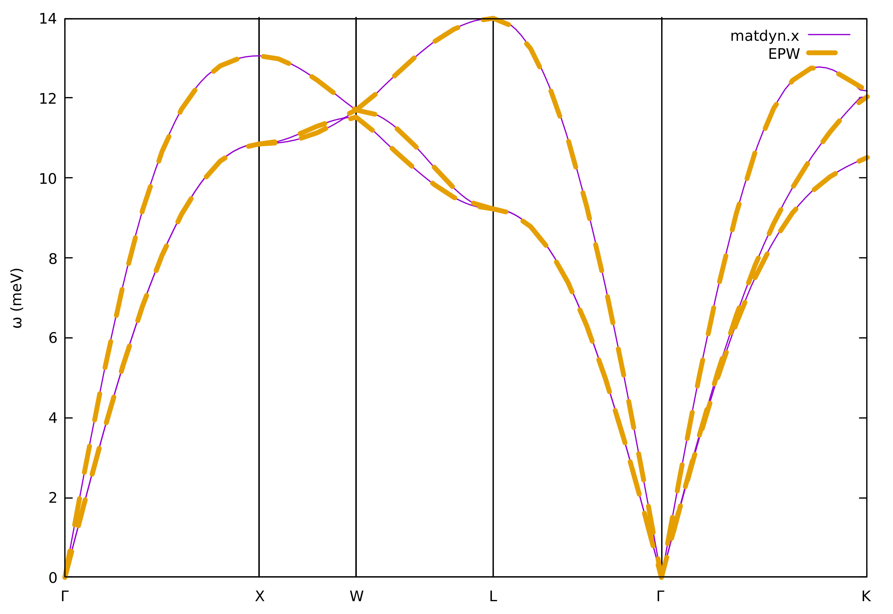
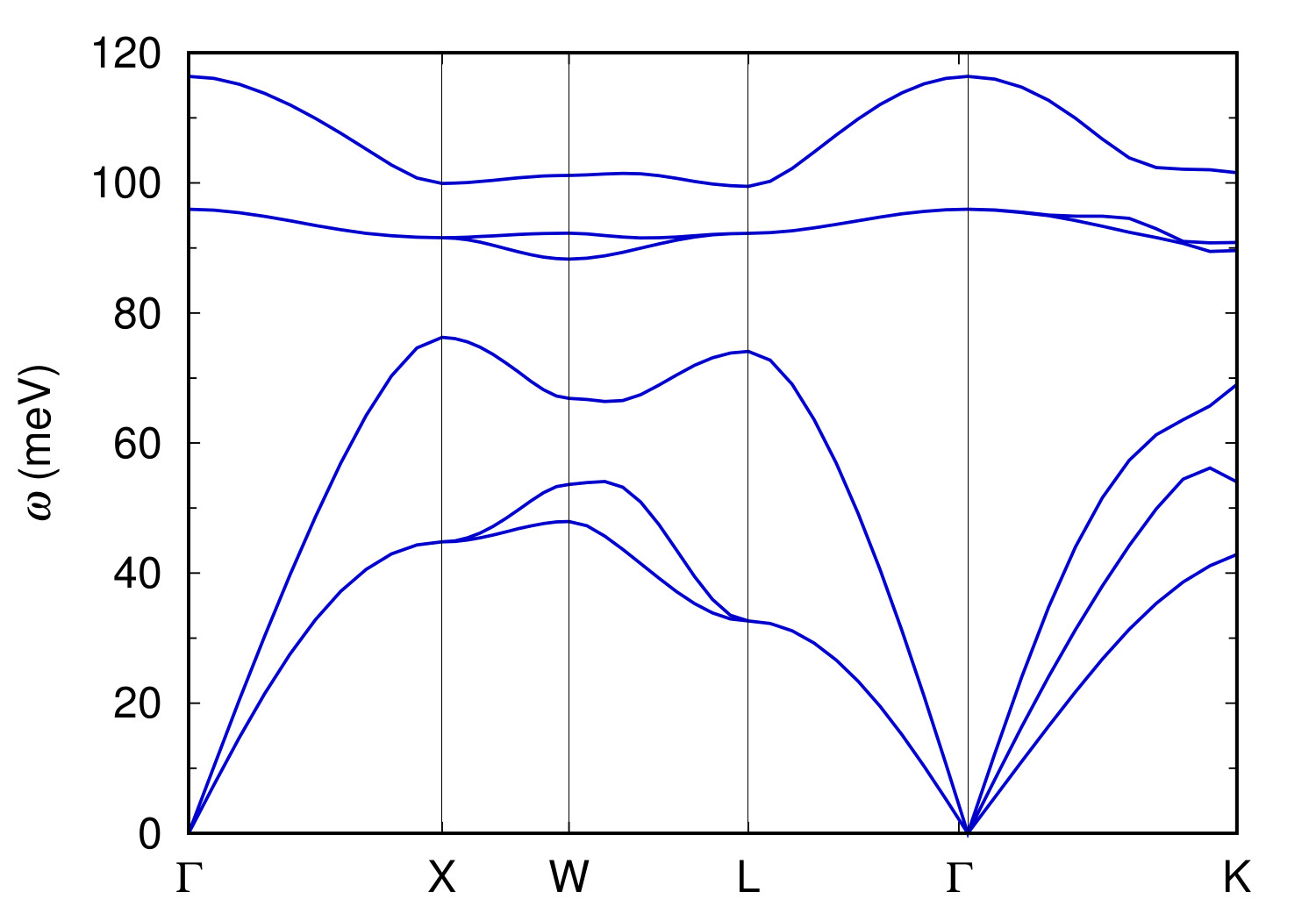
We can also compare the phonon band structures:
$ gnuplot
gnuplot> set terminal x11 enhanced
gnuplot> set encoding utf8
gnuplot> set ylabel "{/Symbol w} (meV)"
gnuplot> set xtics ("{/Symbol G}" 0, "X" 1, "W" 1.5, "L" 2.2071, "{/Symbol G}" 3.0731, "K" 4.1338)
gnuplot> set arrow from 1, graph 0 to 1, graph 1 nohead
gnuplot> set arrow from 1.5, graph 0 to 1.5, graph 1 nohead
gnuplot> set arrow from 2.2071, graph 0 to 2.2071, graph 1 nohead
gnuplot> set arrow from 3.0731, graph 0 to 3.0731, graph 1 nohead
gnuplot> plot "../phonon/pb.freq.gp" u 1:($2/8.06554) w l lw 3 lt 1 title "matdyn.x", \
"" u 1:($3/8.06554) w l lw 3 lt 1 notitle, \
"" u 1:($4/8.06554) w l lw 3 lt 1 notitle, \
"freq.dat" u 1:2 w l lw 3 dt 2 title "EPW"
gnuplot> exit
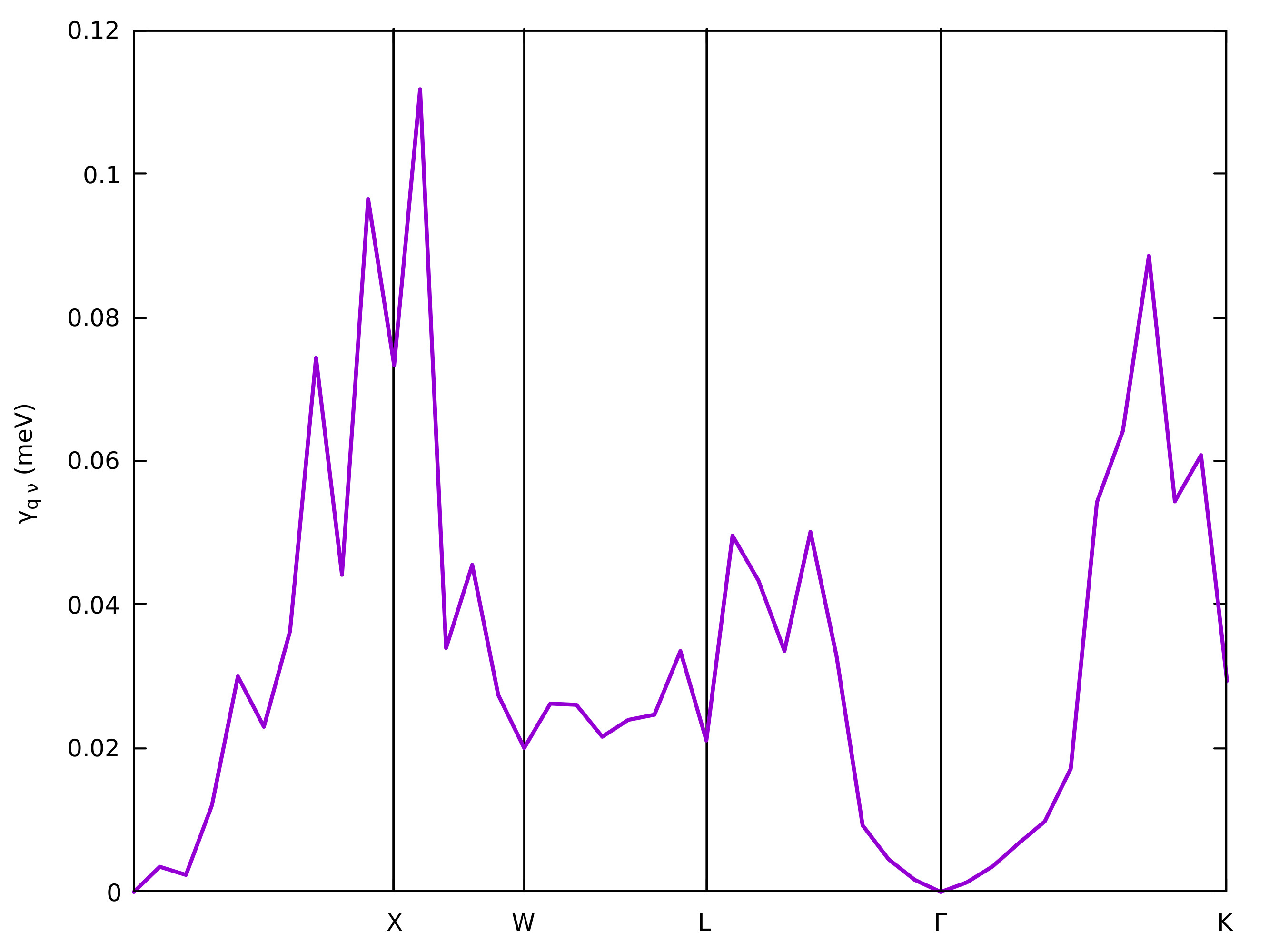
7th step: We now calculate the phonon linewidths
\(\gamma_{\mathbf{q}\nu}\), the imaginary part of the phonon self-energy
\(\Pi_{\mathbf{q}\nu}^{''}\), and the electron-phonon coupling
strength \(\lambda_{\mathbf{q}\nu}\) associated with a specific
phonon mode \(\nu\) and wavevector q within the double-delta
approximation along high-symmetry lines by setting phonselfen=.true.
delta_approx=.true.:
where \(\varepsilon_{\rm F}\) is the Fermi level and the coupling strength is defined as:
where \(N(\varepsilon_{\rm F})\) is the density of states per spin at the Fermi level.
--                                                                                      epw3.in
&inputepw
  prefix      = 'pb',
  amass(1)    = 207.2
  outdir      = './'
  dvscf_dir   = '../phonon/save'

  etf_mem     = 0

  elph        = .true.
  epbwrite    = .false.
  epbread     = .false
  epwwrite    = .false.
  epwread     = .true.

  wannierize  = .false.
  nbndsub     =  4
  bands_skipped = 'exclude_bands = 1-5'
  num_iter    = 300
  dis_win_max = 21
  dis_froz_max= 13.5
  proj(1)     = 'Pb:sp3'

  phonselfen  = .true.
  delta_approx= .true.

  fsthick     = 1     ! eV
  temps       = 0.075 ! K
  degaussw    = 0.2   ! eV

  filqf       = 'pb_band.kpt'
  nkf1         = 20
  nkf2         = 20
  nkf3         = 20

  nk1         = 6
  nk2         = 6
  nk3         = 6
  nq1         = 3
  nq2         = 3
  nq3         = 3
 /
You can see that now the phonon linewidths and coupling strengths are
printed in output for each phonon wavevector \(\mathbf{q}\) and mode
\(\nu\) (lambda___ and gamma___). The sum of
\(\lambda_{\mathbf{q}\nu}\) over all phonon modes, \(\lambda_\mathbf{q}\), is
also written (lambda___( tot )). \(\gamma_{\mathbf{q}\nu}\) and
\(\lambda_{\mathbf{q}\nu}\) are stored in the files
linewidth.phself.XXXK and lambda.phself.XXXK, respectively.
Inspect those files to familiarize yourself with the format and learn
how to plot these quantities. For example, to plot the
\(\mathbf{q}\)-dependent linewidth of the third phonon, you can type in
gnuplot:
$ gnuplot
gnuplot> plot "linewidth.phself.0.075K" u 1:4 every 3::2 w l lw 2
and you should be able to produce a plot like this:
Exercise 2: Semiconducting 3C-SiC
In this exercise we will examine the electron-phonon interaction in semiconducting 3C-SiC which is a polar material where electrons interact with longitudinal optical modes, resulting in a Fröhlich divergence 1/\(|\mathbf{q}|\) divergence of the electron-phonon matrix elements for \(|\mathbf{q}|\) \(\rightarrow\) 0 (PRL 115, 176401 (2015)) as well as a quadrupolar contribution in the long-wavelength limit (PRR 3, 043022 (2021)). Here we start by checking the quality of Wannier interpolation as we did in Exercise 1; then we will see how to correctly interpolate the electron-phonon matrix elements in this case and calculate the electron linewidth.
1st step: Run a self-consistent calculation on a homogeneous \(8\times8\times8\) -point grid and a phonon calculation on a homogeneous \(3\times3\times3\) \(\mathbf{q}\)-point grid using the following inputs and jobscript:
$ cd ../../exercise2
$ cd phonon
$ sbatch job.ph
job.ph
#!/bin/bash
#SBATCH -J myjob              # Job name
#SBATCH -N 1                  # Total # of nodes
#SBATCH --ntasks-per-node 8
#SBATCH -t 01:00:00           # Run time (hh:mm:ss)
#SBATCH -A DMR23030
#SBATCH -p skx
##SBATCH --reservation=NSF_Summer_School_Tue

module list

# Launch MPI code...
export PATHQE=/work2/05193/sabyadk/stampede3/EPWSchool2024/q-e

ibrun $PATHQE/bin/pw.x -nk 4 -in scf.in > scf.out
ibrun $PATHQE/bin/ph.x -nk 4 -in ph.in > ph.out
--                                                                                        scf.in
 &control
    calculation     = 'scf'
    prefix          = 'sic'
    restart_mode    = 'from_scratch'
    pseudo_dir      = '../'
    outdir          = './'
 /
 &system
    ibrav           = 2
    celldm(1)       = 8.237
    nat             = 2
    ntyp            = 2
    ecutwfc         = 30.0
 /
 &electrons
    diagonalization = 'david'
    mixing_beta     = 0.7
    conv_thr        = 1.0d-10
 /
ATOMIC_SPECIES
  Si  28.0855     Si.pz-vbc.UPF
  C   12.01078    C.UPF
ATOMIC_POSITIONS alat
  Si  0.00  0.00  0.00
  C   0.25  0.25  0.25
K_POINTS automatic
8 8 8 0 0 0
--                                                                                         ph.in
&inputph
  prefix   = 'sic'
  fildvscf = 'dvscf'
  ldisp    = .true
  fildyn   = 'sic.dyn.xml'
  nq1=3,
  nq2=3,
  nq3=3,
  tr2_ph   =  1.0d-16
 /
Note that the output of ph.out now contains also the Born effective
charges \(Z^\ast\) and the electronic dielectric constant
\(\epsilon_\infty\):
Electric Fields Calculation

....

End of electric fields calculation

     Dielectric constant in cartesian axis

     (       7.214365306       0.000000000       0.000000000 )
....

     Effective charges (d Force / dE) in cartesian axis

      atom      1   Si
 Ex  (        2.67023        0.00000       -0.00000 )
 ....
q2r.x and matdyn.x with the inputs:-- q2r.in
&input
zasr='simple', fildyn='sic.dyn.xml', flfrc='sic333.fc'
/
--                                                                                     matdyn.in
&input
  asr              = 'simple',
  flfrc            = 'sic333.fc.xml'
  flfrq            = 'sic.freq'
  q_in_band_form   = .true.
  q_in_cryst_coord = .true.
/
  6
  0.000 0.000 0.000  30
  0.500 0.000 0.500  30
  0.500 0.250 0.750  30
  0.500 0.500 0.500  30
  0.000 0.000 0.000  30
  0.375 0.375 0.750  30
You can plot the phonon dispersion using sic.freq.gp.
$ gnuplot
gnuplot> plot for [col=2:7] "sic.freq.gp" using 1:col w l lt 1 notitle
The plot should look like this:
.dyn, .dvscf and patterns files into
a save/ directory as in Exercise 1 using the pp.py script:$ python3 /work2/05193/sabyadk/stampede3/EPWSchool2024/q-e/EPW/bin/pp.py
Enter the prefix of your calculation (sic):
Enter the prefix used for PH calculations (e.g. diam)
sic
4th step: Run a calculation for the direct evaluation of electron-phonon matrix elements along the selected high-symmetry lines using density-functional perturbation theory.
$ cd ../ephline
$ sbatch job.ph
--                                                                                        job.ph
#!/bin/bash
#!/bin/bash
#SBATCH -J myjob              # Job name
#SBATCH -N 1                  # Total # of nodes
#SBATCH --ntasks-per-node 18
#SBATCH -t 01:00:00           # Run time (hh:mm:ss)
#SBATCH -A DMR23030
#SBATCH -p skx
##SBATCH --reservation=NSF_Summer_School_Tue

module list

# Launch MPI code...
export PATHQE=/work2/05193/sabyadk/stampede3/EPWSchool2024/q-e

ibrun $PATHQE/bin/pw.x -nk 18 -in scf.in > scf.out
ibrun $PATHQE/bin/ph.x -nk 18 -in ephline.in > ephline.out
--                                                                                    ephline.in
&inputph
  prefix   = 'sic'
  fildvscf = 'dvscf'
  ldisp    = .true.
  fildyn   = 'sic.dyn.xml'
  tr2_ph   =  1.0d-16
  qplot    = .true.
  q_in_band_form = .true.
  electron_phonon = 'prt'
  kx = 0.0
  ky = 0.0
  kz = 0.0
/
3
  1.0000 0.0000 0.0000 20 # X
  0.0000 0.0000 0.0000 20 # Gamma
 -0.5000 0.5000 0.5000 1  # L
The electron-phonon matrix elements for \(\mathbf{k}\) = \(\Gamma\)
(default) and each \(\mathbf{q}\) along the BZ path are written in the
output of ephline.out, with columns corresponding to each band and
phonon mode. Since electron-phonon matrix elements are gauge-dependent,
an (gauge-invariant) average of their norm over degenerate subspaces of
bands and modes has been performed. If you want to change the wavevector
\(\mathbf{k}\) of the initial state, you can do it by specifying the input
flags of kx, ky, kz (in Cartesian \(2\pi/a\) units).
To extract and plot the electron-phonon matrix elements for the valence-band top (n = m = 4) and a given frequency phonon branch (\(\nu\) = 1 for example), you can type with the eight spaces between digits:
$ grep "4        4        1" ephline.out > data1
$ grep "4        4        3" ephline.out > data3
$ grep "4        4        4" ephline.out > data4
$ grep "4        4        6" ephline.out > data6
where mode index 2 and 5 are degenerate with 1 and 4, respectively. This
data will be processed together with the corresponding data from EPW
for comparison.
EPW and for the Wannier interpolation
of electron-phonon matrix elements along the high-symmetry lines.$ cd ../epw
$ sbatch job.epw1
--                                                                                      job.epw1
#!/bin/bash
#SBATCH -J myjob              # Job name
#SBATCH -N 1                  # Total # of nodes
#SBATCH --ntasks-per-node 8
#SBATCH -t 01:00:00           # Run time (hh:mm:ss)
#SBATCH -A DMR23030
#SBATCH -p skx
##SBATCH --reservation=NSF_Summer_School_Tue

module list

# Launch MPI code...
export PATHQE=/work2/05193/sabyadk/stampede3/EPWSchool2024/q-e

mkdir sic.save
cp ../phonon/sic.save/charge-density.dat sic.save/
cp ../phonon/sic.save/data-file-schema.xml sic.save/

ibrun $PATHQE/bin/pw.x -nk 4 -in nscf.in > nscf.out
ibrun $PATHQE/bin/epw.x -nk 8 -in epw1.in > epw1.out
--                                                                                       nscf.in
 &control
    calculation     = 'nscf'
    prefix          = 'sic'
    pseudo_dir      = '../'
    outdir          = './'
 /
 &system
    ibrav           = 2
    celldm(1)       = 8.237
    nat             = 2
    ntyp            = 2
    ecutwfc         = 30.0
    nbnd            = 4
 /
 &electrons
    diagonalization = 'david'
    mixing_beta     = 0.7
    conv_thr        = 1.0d-10
 /
ATOMIC_SPECIES
  Si  28.0855     Si.pz-vbc.UPF
  C   12.01078    C.UPF
ATOMIC_POSITIONS alat
  Si  0.00  0.00  0.00
  C   0.25  0.25  0.25
K_POINTS crystal
216
  0.00000000  0.00000000  0.00000000  4.629630e-03
  0.00000000  0.00000000  0.16666667  4.629630e-03
  0.00000000  0.00000000  0.33333333  4.629630e-03
...
--                                                                                      epw1.in
&inputepw
  prefix      = 'sic'
  amass(1)    = 28.0855
  amass(2)    = 12.0107
  outdir      = './'
  dvscf_dir   = '../phonon/save'

  elph        = .true.
  epwwrite    = .true.
  epwread     = .false.
  lpolar      = .true.
  vme         = 'dipole'

  wannierize  = .true.
  nbndsub     =  4
  num_iter    = 300
  proj(1)     = 'Si:sp3'

  prtgkk      = .true.

  filqf       = 'path1.dat'
  nkf1        = 1
  nkf2        = 1
  nkf3        = 1

  nk1         = 6
  nk2         = 6
  nk3         = 6
  nq1         = 3
  nq2         = 3
  nq3         = 3
 /
Note that in order to speed up the calculation, we chose to print the
electron-phonon matrix elements for the initial electronic states only
at \(\mathbf{k}\) = \(\Gamma\) (nkf1=nkf2=nkf3=1).
In this calculation, we consider the BZ path of X-\(\Gamma\)-L by
providing the file path1.dat along the same direction as in the
../ephline folder but with more points:
101 cartesian                                                                          path1.dat
    1.0000000000  0.000000000  0.000000000  1.0
    0.9800000000  0.000000000  0.000000000  1.0
    0.9600000000  0.000000000  0.000000000  1.0
    0.9400000000  0.000000000  0.000000000  1.0
    0.9200000000  0.000000000  0.000000000  1.0
    0.9000000000  0.000000000  0.000000000  1.0
    0.8800000000  0.000000000  0.000000000  1.0
    0.8600000000  0.000000000  0.000000000  1.0
....
This file can be generated directly using Wannier90 called in
library mode from EPW or with the following python scrip:
import numpy as np
for ii in np.linspace(1,0,51):
    print( '{:16.10f}  0.000000000  0.000000000  1.0'.format(ii))
for ii in np.linspace(0+0.5/50,0.5,50):
    print( '{:16.10f}  {:16.10f}  {:16.10f}  1.0'.format(-ii,ii,ii))
Note that the printing of interpolated electron-phonon matrix elements
to the output file is activated in EPW with the input variable
prtgkk = .true..
Since 3C-SiC is not a metal, we set lpolar = .true. in order to
correctly treat the long-range interaction in bulk crystals. The
strategy consists in subtracting the long-range component
\(g^\mathcal{L}\) from the full matrix element \(g\) before
interpolation and adding it back after interpolation (see e.g. npj
Comput Mater 9, 156
(2023) for more
details). An analogous strategy is implemented to correctly interpolate
the dynamical matrix including the long-range interactions which result
in the LO-TO splitting.
In EPW, two long-range contributions can be considered: dipoles and
quadrupoles. By default, only the dipoles will be considered when
lpolar = .true.. To include quadrupoles, you need to provide a
quadrupole.fmt file. The file must have that name and be located
in the folder in which you run the calculation. We have taken the
quadrupole value from Table II of Ref. PRR 3, 043022
(2021)
and the quadrupole files (3 lines per atoms) is as follow:
atom   dir       Qxx         Qyy         Qzz         Qyz         Qxz         Qxy
    1     1      0.000000    0.000000    0.000000    6.870000    0.000000    0.000000
    1     2      0.000000    0.000000    0.000000    0.000000    6.870000    0.000000
    1     3      0.000000    0.000000    0.000000    0.000000    0.000000    6.870000
    2     1      0.000000    0.000000    0.000000   -2.440000    0.000000    0.000000
    2     2      0.000000    0.000000    0.000000    0.000000   -2.440000    0.000000
    2     3      0.000000    0.000000    0.000000    0.000000    0.000000   -2.440000
Note : You can compute the quadrupole tensor for your materials via
fitting of the perturbed density or fitting of direct electron-phonon
matrix elements (see
here or
here for
example). Alternatively (easiest option), you can use perturbation
theory and the Abinit code to compute quadrupole tensor, see
https://docs.abinit.org/topics/longwave.
You can verify that quadrupoles are correctly included in the
calculation by looking at the epw1.out where you should find:
------------------------------------
Quadrupole tensor is correctly read:
------------------------------------
atom   dir        Qxx       Qyy      Qzz        Qyz       Qxz       Qxy
  1        x       0.00000   0.00000   0.00000   6.87000   0.00000   0.00000
  1        y       0.00000   0.00000   0.00000   0.00000   6.87000   0.00000
  1        z       0.00000   0.00000   0.00000   0.00000   0.00000   6.87000
  2        x       0.00000   0.00000   0.00000  -2.44000   0.00000   0.00000
  2        y       0.00000   0.00000   0.00000   0.00000  -2.44000   0.00000
  2        z       0.00000   0.00000   0.00000   0.00000   0.00000  -2.44000
The electron-phonon matrix elements for \(\mathbf{k}\) = \(\Gamma\) and
each \(\mathbf{q}\) along the BZ path are written in the output of
epw1.out, with columns corresponding to each band and phonon mode.
Since electron-phonon matrix elements are gauge-dependent, an
(gauge-invariant) average of their norm over degenerate subspaces of
bands and modes has been performed. To extract and plot the
electron-phonon matrix elements for the valence-band top (n = m = 4) and
the phonon branches, as done in the 4th step, you can type with eight
spaces between digits:
$ grep "4        4        1" epw1.out > epwdata1
$ grep "4        4        3" epw1.out > epwdata3
$ grep "4        4        4" epw1.out > epwdata4
$ grep "4        4        6" epw1.out > epwdata6
You can now compare the direct DFPT calculation made before with the interpolated results using gnuplot (assume you connected with X11 support on Frontera and you are in the epw folder):
$ gnuplot
gnuplot> set terminal x11 enhanced
gnuplot> set encoding utf8
gnuplot> set ylabel "|g|_{avg} (meV)" font ",20"
gnuplot> set xtics ("X" 0, "{/Symbol G}" 50, "L" 100) font ",20"
gnuplot> set ytics (0,300,600,900) font ",20"
gnuplot> set arrow from 50, graph 0 to 50, graph 1 nohead
gnuplot> set yrange[0:900]

gnuplot> plot "epwdata1" u 7 w l lw 2 lc rgb "red" title "EPW",\
     "epwdata3" u 7 w l lw 2 lc rgb "red" notitle,\
     "epwdata4" u 7 w l lw 2 lc rgb "red" notitle,\
     "epwdata6" u 7 w l lw 2 lc rgb "red" notitle

gnuplot> replot "../ephline/data1" u ($0*2.5):7 w p pt 5 ps 1.5 lc rgb "black" title "ph.x",\
    "../ephline/data3" u ($0*2.5):7 w p pt 5 ps 1.5 lc rgb "black" notitle,\
    "../ephline/data4" u ($0*2.5):7 w p pt 5 ps 1.5 lc rgb "black" notitle,\
    "../ephline/data6" u ($0*2.5):7 w p pt 5 ps 1.5 lc rgb "black" notitle

gnuplot> exit
Note : We multiply the DFPT x-axis by 2.5 simply because this is the
ratio of number of points computed with EPW.
You should obtain the following figure:
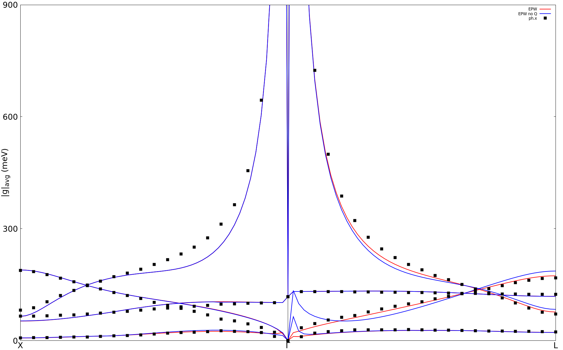
Note that we are also showing the results without quadrupole in that
figure (blue line). You can try to obtain this by simply removing the
quadrupole.fmt file and re-running epw1.in. In addition, note that
the interpolated ones are not fully accurate, since a larger coarse
\(\mathbf{q}\)-grid is needed in order to accurately interpolate the
electron-phonon matrix elements.
lpolar=.false..
Remember to run this test in a new directory, or to run again an
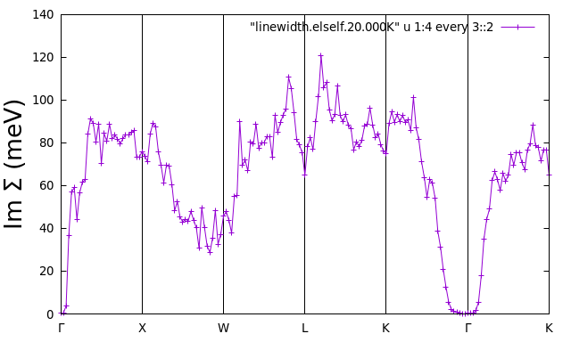
EPW calculation from scratch using lpolar=.true..6th step: We now calculate the linewidths of the valence states in SiC along high-symmetry lines, which correspond to twice the imaginary part of the electron self-energy \(\Sigma_{n\mathbf{k}}^{''}\):
To do so, we need to use the input variable elecselfen = .true., the
\(\mathbf{k}\)-point path, and a homogeneous \(\mathbf{q}\) grid for the
integration.
$ sbatch job.epw2
--                                                                                      job.epw2
#!/bin/bash
#SBATCH -J myjob              # Job name
#SBATCH -N 1                  # Total # of nodes
#SBATCH --ntasks-per-node 8
#SBATCH -t 01:00:00           # Run time (hh:mm:ss)
#SBATCH -A DMR23030
#SBATCH -p skx
##SBATCH --reservation=NSF_Summer_School_Tue

module list

# Launch MPI code...
export PATHQE=/work2/05193/sabyadk/stampede3/EPWSchool2024/q-e

ibrun $PATHQE/bin/epw.x -nk 8 -in epw2.in > epw2.out
--                                                                                       epw2.in
&inputepw
  prefix      = 'sic'
  amass(1)    = 28.0855
  amass(2)    = 12.0107
  outdir      = './'
  dvscf_dir   = '../phonon/save'

  etf_mem     = 0

  elph        = .true.
  epwwrite    = .false.
  epwread     = .true.
  lpolar      = .true.
  vme         = 'dipole'

  wannierize  = .false.
  nbndsub     =  4
  num_iter    = 300
  proj(1)     = 'Si:sp3'

  elecselfen  = .true.
  efermi_read = .true.
  fermi_energy= 9.6

  fsthick     = 7.0
  temps       = 20
  degaussw    = 0.05

  filkf       = 'path2.dat'
  nqf1        = 20
  nqf2        = 20
  nqf3        = 20

  nk1         = 6
  nk2         = 6
  nk3         = 6
  nq1         = 3
  nq2         = 3
  nq3         = 3
 /
efermi_read = .true. and fermi_energy=9.6 (just above the
valence-band top). Progression iq (fine) = 50/ 8000
Progression iq (fine) = 100/ 8000
...
...
Average over degenerate eigenstates is performed
Temperature: 20.000K
WARNING: only the eigenstates within the Fermi window are meaningful
ik = 1 coord.: 0.0000000 0.0000000 0.0000000
-------------------------------------------------------------------
E( 2 )= -0.2406 eV Re[Sigma]= 96.661664 meV Im[Sigma]= 0.240285 meV Z= 0.860491 lam= 0.162127
E( 3 )= -0.2406 eV Re[Sigma]= 96.661664 meV Im[Sigma]= 0.240285 meV Z= 0.860491 lam= 0.162127
E( 4 )= -0.2406 eV Re[Sigma]= 96.661664 meV Im[Sigma]= 0.240285 meV Z= 0.860491 lam= 0.162127
-------------------------------------------------------------------
...
Note that the electron energies are now reported with respect to
\(E_{\rm F}\). Moreover, the self-energy for the first valence band
is not computed since fsthick is 7 eV. To plot the linewidths you
can use the file linewidth.elself that has been created. For
example, Im\(\Sigma\) for the highest valence band should look
like:
$ gnuplot
gnuplot> set terminal x11 enhanced
gnuplot> set encoding utf8
gnuplot> set ylabel "Im {/Symbol S} (meV)" font ",20"
gnuplot> set xtics ("{/Symbol G}" 1, "X" 31, "W" 61, "L" 91, "K" 121, "{/Symbol G}" 151, "K" 181)
gnuplot> set arrow from 31, graph 0 to 31, graph 1 nohead
gnuplot> set arrow from 61, graph 0 to 61, graph 1 nohead
gnuplot> set arrow from 91, graph 0 to 91, graph 1 nohead
gnuplot> set arrow from 121, graph 0 to 121, graph 1 nohead
gnuplot> set arrow from 151, graph 0 to 151, graph 1 nohead
gnuplot> set yrange[0:140]
gnuplot> plot "linewidth.elself.20.000K" u 1:4 every 3::2 w lp
gnuplot> exit
iverbosity = 3 in the input. The file
linewidth.elself will then contain the mode-resolved linewidths.
Can you tell which phonon has the largest contribution and why?Try increasing the \(\mathbf{q}\) grid, and also using a random set of \(\mathbf{q}\) points: you will see the linewidths are not well converged yet. For polar materials it is indeed more difficult to converge Brillouin-zone integrals, due to the \(1/|\mathbf{q}|\) divergence of the Fröhlich matrix elements.
Extra exercise
Repeat the 4th and 6th steps of Exercise 2 with the wavevector \(\mathbf{k}\) of the initial state set to (-0.5,-1.0,0.0) (in Cartesian 2\(\pi/a\) units).
Hint: You can proceed in the following way:
$ cd ephline
* Modify the following lines in ephline.in:
! kx = 1.2500000
! ky = 0.8750000
! kz = 1.2500000
$ sbatch job.ph
$ cd ../epw/
* Modify the following lines in epw1.in:
nkf1 = 1
nkf2 = 1
nkf3 = 1
* And create a necessary file.
$ sbatch job.epw1