Anharmonic special displacement method
04/08/2026
Note
Hands-on based on QE-v7.3.1 and EPW-v5.9
Note
It is perfectly reasonable to obtain ZG displacements that differ from those reported in this tutorial. These differences arise from numerical accuracy in the phonon calculations and from the gauge freedom of the vibrational modes: modes obtained by diagonalizing the dynamical matrix may differ by a phase factor (or by a unitary transformation in the case of degeneracy) when computed on different HPC systems. The final results, within reasonable accuracy, are not affected by these differences.
In this tutorial we will learn to use the core capabilities of the ZG.x code for applying the anharmonic special displacement method (ASDM), and how to combine it with standard Density Functional Theory (DFT) calculations for evaluating anharmonicity and anharmonic electron-phonon properties.
Prerequisites
This tutorial assumes that Quantum ESPRESSO and EPW have already been downloaded and compiled.
If you have not yet completed these steps,
please follow the Installation and setup tutorial before continuing.
The examples below also assume that the environment variables used to run the executables
(such as $QE, $RUN_PW, and $RUN_ZG) have been defined as described in the Installation and setup .
Note that variables defined with export only apply to the current terminal session.
If you compiled the code previously but are starting a new session,
you may need to redefine the run variables following the instructions in Defining run commands.
If the setup tutorial has been followed in the current session, the commands below should work directly in your terminal.
Download input files
Download the tutorial tarball (tutorial03.tar.gz) from this link and untar.
You are advised to prepare the following script file, e.g. script.sh:
#!/bin/bash
#SBATCH --job=ASDM
#SBATCH --nodes=1
#SBATCH --ntasks-per-node=48
#SBATCH --time=01:00:00
#SBATCH --account=
#SBATCH --partition=
#SBATCH --reservation=
# Load Modules
#
QE=/path_to/q-e/bin # path to "bin" of q-e
export RUN_PW="mpirun -np 4 $QE/pw.x"
export RUN_PH="mpirun -np 4 $QE/ph.x"
export RUN_Q2R="$QE/q2r.x"
export RUN_MATDYN="$QE/matdyn.x"
export RUN_ZG="$QE/ZG.x"

cd $PWD
For each calculation, pass the command at the bottom of the script and submit the job, e.g. sbatch script.sh. Also set the following environment variable in your shell:
export QE=/path_to/q-e/bin/
All necessary executables and the ZG module are compiled with EPW, i.e. with make epw. To use local executables go to q-e/EPW/ZG/src/local and type ./compile_ifort.sh. The description of all input flags is available in this link .
Exercise 1: Anharmonic lattice dynamics (zirconium)
Exercise 2: Anharmonic electron-phonon coupling (PbTe)
Exercise 3: Anharmonic electron-phonon coupling in polymorphous systems (CsPbBr\(_3\))
Exercise 1
Note: To perform ASDM calculations, one is advised to complete first SDM: Exercise 1.
In this exercise we will learn how to calculate temperature-dependent anharmonic phonons of Zr at \(T=1188\) K using \(2\times2\times2\) ZG-supercells and the anharmonic special displacement method (ASDM). The ASDM combines the special displacement method with the self-consistent phonon (SCP) theory; details for the theory related to this exercise please refer to Refs. [Phys. Rev. B 108, 035155 (2023) ] and [D. Hooton, LI. a new treatment of anharmonicity in lattice thermodynamics: I, London Edinburgh Philos. Mag. J. Sci. 46, 422 (1955)]. The main aim is to find the effective matrix of IFCs that best describes anharmonicity in the potential energy surface. For this reason we minimize the trial free energy with respect to the matrix of IFCs which requires, essentially, to evaluate self-consistently the IFCs.
In the following we are going to show how to calculate IFCs self-consistently by performing a series of finite difference calculations.
First, untar the tutorial, go to the directory exercise1 and copy the following input files in your workdir:
cd $SCRATCH
tar -xvf tutorial03.tar.gz; cd tutorial03/exercise1
mkdir workdir; cd workdir
cp ../inputs/Zr.upf ../inputs/scf.in ../inputs/ph.in .
cp ../inputs/q2r.in ../inputs/matdyn.in .
Below we provide the scf.in file:
scf.in
&control
        calculation='scf'
        restart_mode='from_scratch'
        prefix = 'scf'
        outdir='./'
        pseudo_dir='./'
        verbosity='high'
/
&system
        ibrav=3
        nat=1
        ntyp=1
        ecutwfc=  30
        A = 3.51695
        occupations = 'smearing'
        smearing='gaussian',
        degauss=0.005d0
/
&electrons
        diagonalization='david'
        mixing_mode='plain'
        mixing_beta=0.7
        conv_thr=1e-7
/
ATOMIC_SPECIES
Zr 91.224 Zr.upf
K_POINTS {automatic}
6 6 6 0 0 0
ATOMIC_POSITIONS (crystal)
Zr 0.0 0.0 0.0
Note: Gaussian smearing for the occupations since Zr is a metal. For speed up we use a small energy cutoff of 30 Ry.
Step 1
Run a self-consistent calculation for Zr in the workdir.
$RUN_PW -nk 4 < scf.in > scf.out
Step 2
Run a ph.x calculation on a homogeneous \(3\times3\times3\) \(\mathbf{q}\)-point grid using the input:
ph.in
&inputph
   amass(1)= 91.224,
   prefix = 'scf'
   outdir = './'
   verbosity = 'high'
   ldisp = .true.
   fildyn = 'Zr.dyn'
   tr2_ph = 1.0d-14
   nq1 = 3
   nq2 = 3
   nq3 = 3
/
$RUN_PH -nk 4 < ph.in > ph.out
This will generate 4 Zr.dynX output files containing the dynamical matrix calculated for each irreducible \(\mathbf{q}\)-point. The list of irreducible \(\mathbf{q}\)-points is written in the Zr.dyn0 file.
Step 3
Run a q2r.x calculation to obtain the interatomic force constants (IFC)
file using the input:
q2r.in
&input
 fildyn='Zr.dyn', zasr='crystal', flfrc = 'Zr.333.fc'
/
$RUN_Q2R < q2r.in > q2r.out
This will generate Zr.333.fc which contains the harmonic IFCs.
Step 4
Run a matdyn.x calculation to obtain the harmonic phonon dispersion:
matdyn.in
&input
    &input
    asr='all', amass(1)= 91.224,
    flfrc='Zr.333.fc', fldyn=' ', flfrq='Zr_harm.freq', fleig=' ', q_in_cryst_coord = .true.
    q_in_band_form = .true.
/
5
 0.00   0.00   0.00 100
 0.50   0.50   0.50 100
 0.75   0.25  -0.25 100
 0.00   0.00   0.00 100
 0.50   0.50   0.00 1
$RUN_MATDYN < matdyn.in > matdyn.out
$QE/plotband.x
Input file > Zr_harm.freq
Reading    3 bands at    401 k-points
Range: -131.7354  166.3357eV  Emin, Emax, [firstk, lastk] > -200 200
high-symmetry point:  0.0000 0.0000 0.0000   x coordinate   0.0000
high-symmetry point:  0.0000 0.0000 1.0000   x coordinate   1.0000
high-symmetry point:  0.5000 0.5000 0.5000   x coordinate   1.8660
high-symmetry point:  0.0000 0.0000 0.0000   x coordinate   2.7321
high-symmetry point:  0.0000 0.5000 0.5000   x coordinate   3.4392
output file (gnuplot/xmgr) > Zr_harm_ph_dispersion.xmgr
bands in gnuplot/xmgr format written to file Zr_harm_ph_dispersion.xmgr
output file (ps) >
stopping ...
matdyn.x will generate Zr_harm.freq which contains the harmonic phonon frequencies. Then we combine Zr_harm.freq with plotband.x to obtain Zr_harm_ph_dispersion.xmgr in gnuplot/xmgr format for the harmonic phonon dispersion. To plot the phonon dispersion type:
cp Zr_harm_ph_dispersion.xmgr ../gnuplot/.
cd ../gnuplot/; gnuplot gp_coms_harm.p; evince Zr_harm_ph_dispersion.pdf
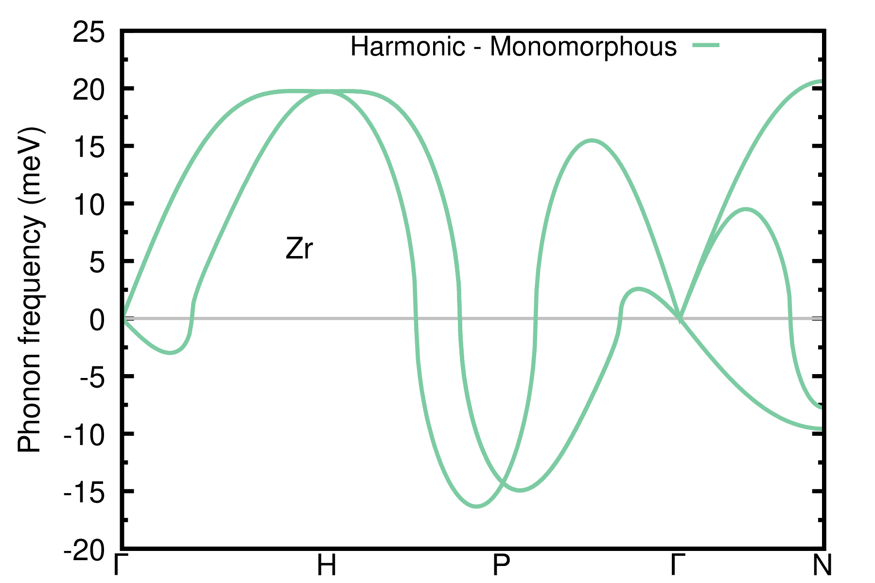
Is the matrix of IFCs positive definite (i.e. all phonon frequencies are positive)? Unlike Si phonon dispersion in SDM: Exercise 1, the answer is no and the phonon dispersion exhibits severe instabilities. Here the harmonic approximation is not enough since anharmonic effects are important in Zr. To treat anharmonicity we are going to use the ASDM in the following.
The starting point of the ASDM for obtaining self-consistent phonons is a crucial step towards convergence and stability. This is because the SCP theory is designed to work with positive definite IFCs matrices. Although one could employ the harmonic phonons as a starting point (and neglect imaginary phonons), we strongly suggest the use of stable phonons as a starting point. For systems with a double well potential like Zr, well-defined dispersions can be obtained by exploring the ground state polymorphous structure, i.e a low-symmetry structure whose energy corresponds to a minimum of the potential energy surface [see also Ref. Phys. Rev. B 101, 155137 (2020)].
In the following we are going to show how to obtain the ground state polymorphous network of Zr and its stable phonons. If you have skipped the steps above, you can copy the harmonic IFCs file from inputs into workdir:
cd ../workdir; cp ../inputs/Zr.333.fc .
Step 5
Run an A_ZG calculation using the input:
ZG_1.in
&input
   asr='all', amass(1)= 91.224, flfrc='Zr.333.fc'
   flscf = 'scf.in'
   atm_zg(1) = 'Zr',
   T = 0
   dim1 = 2, dim2 =2, dim3 =2, incl_qA = .true.
   compute_error = .true., synch = .true., error_thresh = 0.2
   ASDM = .true.
/
&A_ZG
   poly = .true.
   poly_fd_forces = .false.
/
Note: The \({\bf q}\)-point grid (nq1 \(\times\) nq2 \(\times\) nq3) used to obtain the initial dynamical matrices should not be necessarily the same with the supercell size (dim1 \(\times\) dim2 \(\times\) dim3). In particular, dimX is independent of nqX, since ZG.x takes advantage of Fourier interpolation as implemented in matdyn.x; thus any size of ZG configuration can be generated from Zr.333.fc.
cp ../inputs/ZG_1.in .
$RUN_ZG < ZG_1.in > ZG_1.out
The input format of &input list in ZG_1.in is the same as we have seen in SDM: Exercise 1. We remark that here we are using a \(2 \times 2 \times2\) supercell and therefore incl_qA = .true.. The temperature is set initially to T = 0, since we want to explore the polymorphous geometry. Line 7 contains the flag ASDM which enables the ASDM procedure and allows the code to read the input variables in the list &A_ZG. At this step we ask the code by turning poly = .true. to generate the input file for performing a coordinates’ optimization of the structure that will lead to the polymorphous geometry. Apart from the standard ZG.x output files described in SDM: Exercise 1, the code now prints ZG-relax.in. This file contains displaced coordinates of the atoms away from their high-symmetry positions (that define the monomorphous network) in a \(2 \times 2 \times 2\) supercell using ZG displacements.
The file ZG-relax.in is also provided here:
ZG-relax.in
&control
  calculation = relax
  restart_mode = 'from_scratch'
  prefix = 'ZG-relax'
  pseudo_dir = './'
  outdir = './'
  tprnfor=.true.
  disk_io = 'none'
  forc_conv_thr = 1.0D-5
  nstep = 300
/
&system
  ibrav = 0
  nat =    8
  ntyp =    1
  ecutwfc =  30.00
  occupations = 'smearing'
  smearing = 'gaussian'
  degauss =   0.5D-02
/
&electrons
  diagonalization = 'david'
  mixing_mode= 'plain'
  mixing_beta = 0.70
  conv_thr =   0.1D-06
/
&ions
  ion_dynamics = 'bfgs'
/
ATOMIC_SPECIES
   Zr   91.224 Zr.upf
K_POINTS automatic
   3   3   3   0   0   0
CELL_PARAMETERS (angstrom)
      3.51695000      3.51695000      3.51695000
     -3.51695000      3.51695000      3.51695000
     -3.51695000     -3.51695000      3.51695000
ATOMIC_POSITIONS (angstrom)
...
Note: Cell paramaters, number of atoms, k-grid, and atomic coordinates have been modified automatically based on the supercell dimensions. The code will always generate the lattice information in angstroms.
Step 6
Run nuclei coordinates optimization for Zr with the nuclei at their ZG harmonic coordinates (for \(T = 0.00\) K) in the \(2 \times 2 \times 2\) supercell.
mpirun -np 42 $QE/pw.x -nk 14 < ZG-relax.in > ZG-relax.out
The calculation should take around 4.5 minutes. Meanwhile you can check how the total energy evolves by typing grep ! ZG-relax.out. Can you compare the total energy of the relaxed polymorphous structure with the one of the monomorphous structure (unit cell calculation in scf.out)? The polymorpous network is more stable by 22 meV/f.u. If you calculate an energy lowering much less than this value, then (i) increase the initial temperature, e.g. T = 300 in ZG_1.in, (ii) remove file ZG-relax.out, and (iii) repeat the process. A higher temperature increases the phonon population, leading to larger atomic displacements. This can facilitate the exploration of polymorphous structures by preventing the atoms from returning to their high-symmetry positions.
Step 7
Run an A_ZG calculation using the same input file.
cp ../inputs/ZG_1.in ZG_2.in
$RUN_ZG < ZG_2.in > ZG_2.out
The code now will search for the output file ZG-relax.out, read the relaxed final coordinates, and apply finite differences. This will generate ZG-scf_poly_iter_00_XXXX.in files corresponding to the scf inputs for evaluating the IFCs of the polymorphous network by finite differences. The default displacement on each atom is 0.01058 Å , (i.e. 0.02 Bohr). One can change the default value by specifying a value in Å, using the flag fd_displ under the namelist &A_ZG.
Step 8
Run scf calculations for files ZG-scf_poly_iter_00_XXXX.in and save all scf outputs in fd_forces directory.
file=ZG-scf_poly_iter_00
mkdir fd_forces/
for i in {0001..0048}; do
  mkdir $i
  cd $i
  cp ../Zr.upf .
  mv ../"$file"_"$i".in .
  mpirun -np 42 $QE/pw.x -nk 14 < "$file"_"$i".in > "$file"_"$i".out
  mv "$file"_"$i".out ../fd_forces/.
  rm Zr.upf
  cd ../
done
Each scf run should take around 3 seconds and the total calculation around 4 minutes. In the meantime, you can revisit the tutorial slides to refresh the ASDM procedure.
Step 9
Run an A_ZG calculation using the same input file but turn the flag poly_fd_forces = .true..
cp ../inputs/ZG_3.in ZG_3.in
$RUN_ZG < ZG_3.in > ZG_3.out
ZG_3.in is also provided:
ZG_3.in
&input
   asr='all', amass(1)= 91.224, flfrc='Zr.333.fc'
   flscf = 'scf.in'
   atm_zg(1) = 'Zr',
   T = 0
   dim1 = 2, dim2 =2, dim3 =2, incl_qA = .true.
   compute_error = .true., synch = .true., error_thresh = 0.3
   ASDM = .true.
/
&A_ZG
   poly = .true.
   poly_fd_forces = .true.
   incl_epsil = .false.
/
The code now will read all the forces from the files ZG-scf_poly_iter_00_XXXX.out in fd_forces directory and evaluate the IFCs of the polymorphous structure. Apart from the standard ZG.x output files, the code now prints: (i) FORCE_CONSTANTS_poly_iter_00 which contains the IFCs in the same format as phonopy, (ii) FORCE_CONSTANTS_sym_poly_iter_00 which contains the symmetrized IFCs (i.e. after applying all symmetry operations of the crystal), and (iii) poly_iter_00.fc which contains the symmetrized IFCs in the same format as q2r.x output, ready to be used for the next ASDM iteration. You can check the symmetries found by the code using grep "Sym." ZG_3.out or read ZG_3.out directly. For systems where the dielectric constant and Born effective charges are not zero, one may include this information in the XXXX.fc file by setting incl_epsil = .true.. Note that for including the non-analytic contribution to the dynamical matrix one needs to set na_ifc = .true. for the next ZG iteration run (&input list). This is because IFCs are evaluated by finite differences instead of DFPT. The same flag is also necessary for obtaining the phonon dispersion with matdyn.x; if not included the calculation will lead to erroneous results.
Step 10
Run a matdyn.x calculation to obtain the harmonic phonons of the Zr polymorphous network:
cp ../inputs/matdyn_poly.in .
$RUN_MATDYN < matdyn_poly.in > matdyn_poly.out
$QE/plotband.x
matdyn.x will generate Zr_poly.freq which contains the harmonic phonon frequencies of the Zr polymorphous network. Then combine Zr_poly.freq with plotband.x to create the phonon dispersion file Zr_poly_ph_dispersion.xmgr as before. To plot the new phonon dispersion type:
cp Zr_poly_ph_dispersion.xmgr ../gnuplot/.
cd ../gnuplot/; gnuplot gp_coms_poly.p; evince Zr_poly_ph_dispersion.pdf
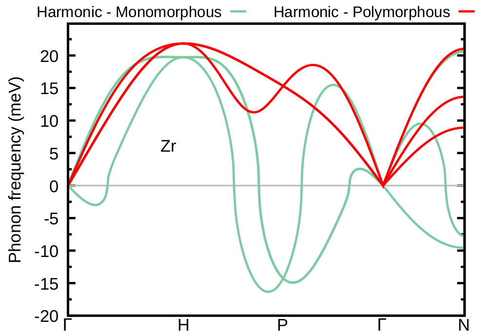
The plot is provided below. Now the matrix of IFCs is positive definite (i.e. all phonon frequencies are positive) and we are ready to account for anharmonicity via the ASDM using as a starting point the symmetrized IFCs of the Zr polymorphous network.
Step 11
Run an A_ZG calculation using the input file:
ZG_4.in
&input
   asr='all', amass(1)= 91.224, flfrc='poly_iter_00.fc'
   flscf = 'scf.in'
   atm_zg(1) = 'Zr',
   T = 1188
   dim1 = 2, dim2 =2, dim3 =2, incl_qA = .true.
   compute_error = .true., synch = .true., error_thresh = 0.3
   ASDM = .true.
/
&A_ZG
   iter_idx = 1
   apply_fd = .true.
/
Note: This is essentially the first iteration indicated by iter idx. The file of IFCs is now flfrc='poly iter 00.fc' and the target temperature is \(T=1188\) K.
cd ../workdir; cp ../inputs/ZG_4.in ZG_4.in
$RUN_ZG < ZG_4.in > ZG_4.out
This will generate a ZG configuration on which finite differences is applied after setting the flag apply_fd = .true.. The scf files are ZG-scf_1188.00K_iter_01_XXXX.in to be used for the evaluation of the temperature-dependent IFCs of the ZG configuration generated for \(T=1188\) K.
Step 12
Run scf calculations for files ZG-scf_1188.00K_iter_01_XXXX.in and save all scf outputs in the directory fd_forces. The script below is as before but with a new name for file variable.
file=ZG-scf_1188.00K_iter_01  # note that only the filename changes
# mkdir fd_forces/
for i in {0001..0048}; do
  # mkdir $i
  cd $i
  cp ../Zr.upf .
  mv ../"$file"_"$i".in .
  mpirun -np 42 $QE/pw.x -nk 14 < "$file"_"$i".in > "$file"_"$i".out
  mv "$file"_"$i".out ../fd_forces/.
  rm Zr.upf
  cd ../
done
Each scf run should take around 3 seconds and the total calculation around 4.5 minutes. We can use this time for some questions.
Step 13
Run an A_ZG calculation using the input file:
ZG_5.in
&input
   asr='all', amass(1)= 91.224, flfrc='poly_iter_00.fc'
   flscf = 'scf.in', atm_zg(1) = 'Zr',
   T = 1188
   dim1 = 2, dim2 =2, dim3 =2, incl_qA = .true.
   compute_error = .true., synch = .true., error_thresh = 0.3
   ASDM = .true.
/
&A_ZG
   iter_idx0 = 0, iter_idx = 1
   apply_fd = .false.
   read_fd_forces = .true.
   mixing = .true.
   incl_epsil = .false.
/
Note: The flag apply_fd is set to .false. since apply_fd and read_fd_forces cannot be both .true..
cp ../inputs/ZG_5.in ZG_5.in
$RUN_ZG < ZG_5.in > ZG_5.out
With the flag read_fd_forces = .true. the code reads all the forces from files ZG-scf_1188.00K_iter_01_XXXX.out in the folder fd_forces and evaluates the IFCs of the ZG configuration. If one scf calculation is not successful, then the code will complain and print the error:
Error in routine ZG (XXXX):
forces in file are missing ...
Here XXXX will be replaced by the code with the file index of the unsuccessful calculation.
If all calculations run successfully, the code evaluates the IFCs using the finite differences formula and prints the following new files related to the first iteration: (i) FORCE_CONSTANTS_1188.00K_iter_01, (ii) FORCE_CONSTANTS_sym_1188.00K_iter_01 and (iii) 1188.00K_iter_01.fc which contains the symmetrized IFCs in the same q2r.x output format, ready to be used for the next ASDM iteration. Here, we set the flag mixing = .true., so that iterative mixing of the IFCs is performed. The input variables iter_idx0 and iter_idx denote the initial and final index of iterations, respectively, for which mixing of IFCs is performed.
Step 14
Run matdyn.x to obtain the temperature-dependent anharmonic phonons of the first iteration:
cp ../inputs/matdyn_01.in .
$RUN_MATDYN < matdyn_01.in > matdyn_01.out
$QE/plotband.x
matdyn.x will generate Zr_01.freq which contains the temperature-dependent anharmonic phonon frequencies of Zr at the first iteration. Then combine Zr_01.freq with plotband.x to create the phonon dispersion file Zr_01_ph_dispersion.xmgr as before. To plot the new phonon dispersion and compare with the previous results type:
cp Zr_01_ph_dispersion.xmgr ../gnuplot/.
cd ../gnuplot/; gnuplot gp_coms_iter_01.p; evince Zr_01_ph_dispersion.pdf
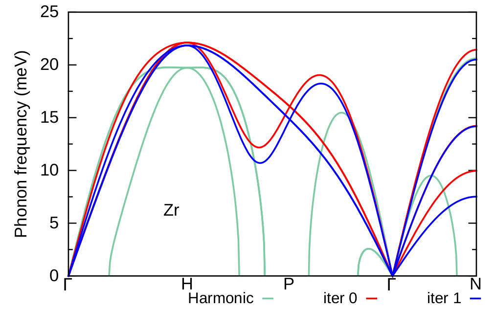
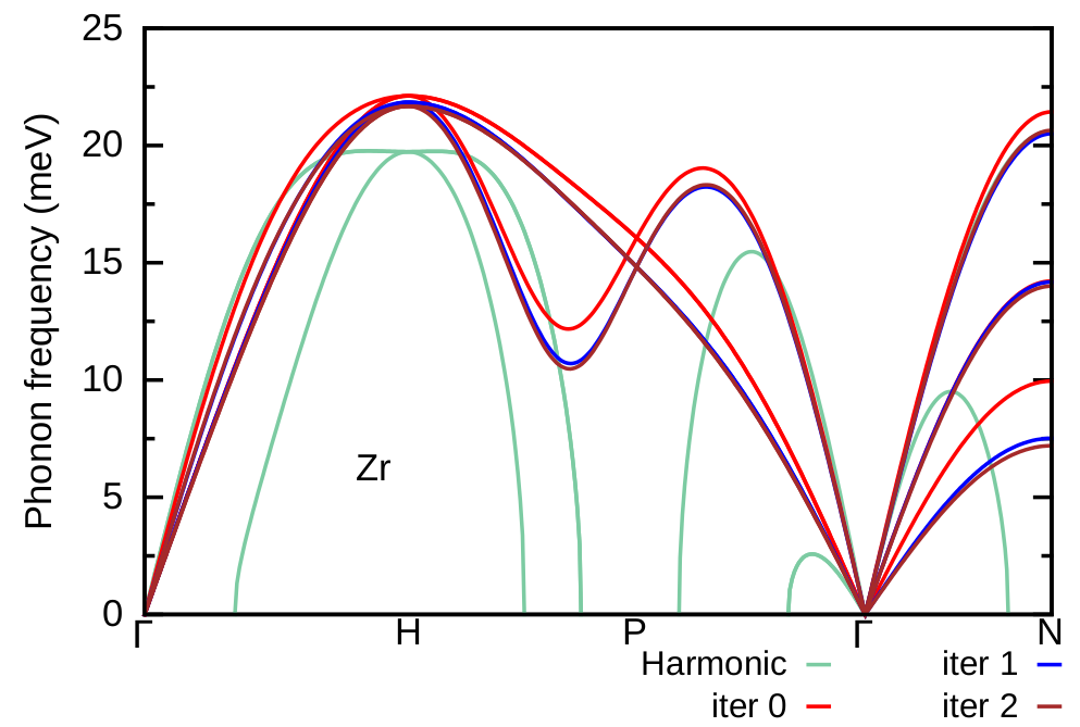
Here, we compare the phonon dispersion of Zr at \(T=1188\) K obtained at the first iteration (blue) with the phonon dispersion of the polymorphous network (red) and the harmonic phonon dispersion (green). As we can see the result from the first iteration follows a similar trend with the one calculated for the polymorphous network. In the following we proceed to the second iteration and re-evaluate the phonon dispersion of Zr at \(T=1188\) K starting from the IFCs of the previous iteration.
Step 15
Run an A_ZG calculation using the input file:
ZG_6.in
&input
   asr='all', amass(1)= 91.224, flfrc='1188.00K_iter_01.fc'
   flscf = 'scf.in'
   atm_zg(1) = 'Zr',
   T = 1188
   dim1 = 2, dim2 =2, dim3 =2, incl_qA = .true.
   compute_error = .true., synch = .true., error_thresh = 0.35
   ASDM = .true.
/
&A_ZG
   iter_idx = 2
   apply_fd = .true.
/
cd ../workdir; cp ../inputs/ZG_6.in ZG_6.in
$RUN_ZG < ZG_6.in > ZG_6.out
This will generate a new ZG configuration and the scf files ZG-scf_1188.00K_iter_02_XXXX.in to be used for the evaluation of the temperature-dependent IFCs of the second iteration.
Step 16
Run scf calculations for files ZG-scf_1188.00K_iter_02_XXXX.in and save all scf outputs in the folder fd_forces.
file=ZG-scf_1188.00K_iter_02  # note that only the index changes
# mkdir fd_forces/
for i in {0001..0048}; do
  # mkdir $i
  cd $i
  cp ../Zr.upf .
  mv ../"$file"_"$i".in .
  mpirun -np 42 $QE/pw.x -nk 14 < "$file"_"$i".in > "$file"_"$i".out
  mv "$file"_"$i".out ../fd_forces/.
  rm Zr.upf
  cd ../
done
Step 17
Run an ASDM calculation using the input file:
ZG_7.in
&input
   asr='all', amass(1)= 91.224, flfrc='1188.00K_iter_01.fc'
   flscf = 'scf.in', atm_zg(1) = 'Zr',
   T = 1188
   dim1 = 2, dim2 =2, dim3 =2, incl_qA = .true.
   compute_error = .true., synch = .true., error_thresh = 0.3
   ASDM = .true.
/
&A_ZG
   iter_idx0 = 0, iter_idx = 2
   apply_fd = .false.
   read_fd_forces = .true.
   mixing = .true.
   incl_epsil = .false.
/
cp ../inputs/ZG_7.in ZG_7.in
$RUN_ZG < ZG_7.in > ZG_7.out
The code will read all the forces from the files ZG-scf_1188.00K_iter_02_XXXX.out in fd_forces and evaluate the IFCs of the new ZG configuration. The code now prints all files related to the second iteration: (i) FORCE_CONSTANTS_1188.00K_iter_02, (ii) FORCE_CONSTANTS_sym_1188.00K_iter_02 and (iii) 1188.00K_iter_02.fc. Mixing is performed between the current and all previous IFCs matrices as specified by the input variables iter_idx0 and iter_idx. We found that for the current system convergence is achieved faster. Instead, one can perform mixing between consecutive iterations (current and previous iteration) by choosing appropriately iter_idx0 and iter_idx. In any case the converged result should be similar.
Step 18
Run a matdyn.x calculation to obtain the temperature-dependent anharmonic
phonons at the second iteration:
cp ../inputs/matdyn_02.in .
$RUN_MATDYN < matdyn_02.in > matdyn_02.out
$QE/plotband.x
matdyn.x will generate Zr_02.freq which contains the temperature-dependent anharmonic phonon frequencies of Zr at the second iteration. Then combine Zr_02.freq with plotband.x to create the phonon dispersion file Zr_02_ph_dispersion.xmgr as before. To plot the new phonon dispersion and compare with the previous results type:
cp Zr_02_ph_dispersion.xmgr ../gnuplot/.
cd ../gnuplot/; gnuplot gp_coms_iter_02.p; evince Zr_02_ph_dispersion.pdf
Here, we compare the phonon dispersion of Zr at \(T=1188\) K obtained at the second iteration (brown) with the one at first iteration (blue), the phonon dispersion of the polymorphous network (red), and the harmonic phonon dispersion (green). As we can see the result at the second iteration is almost converged. One can repeat further iterative steps to check convergence.
As a homework repeat the previous steps for the third and fourth iterations. The results should look like the following:
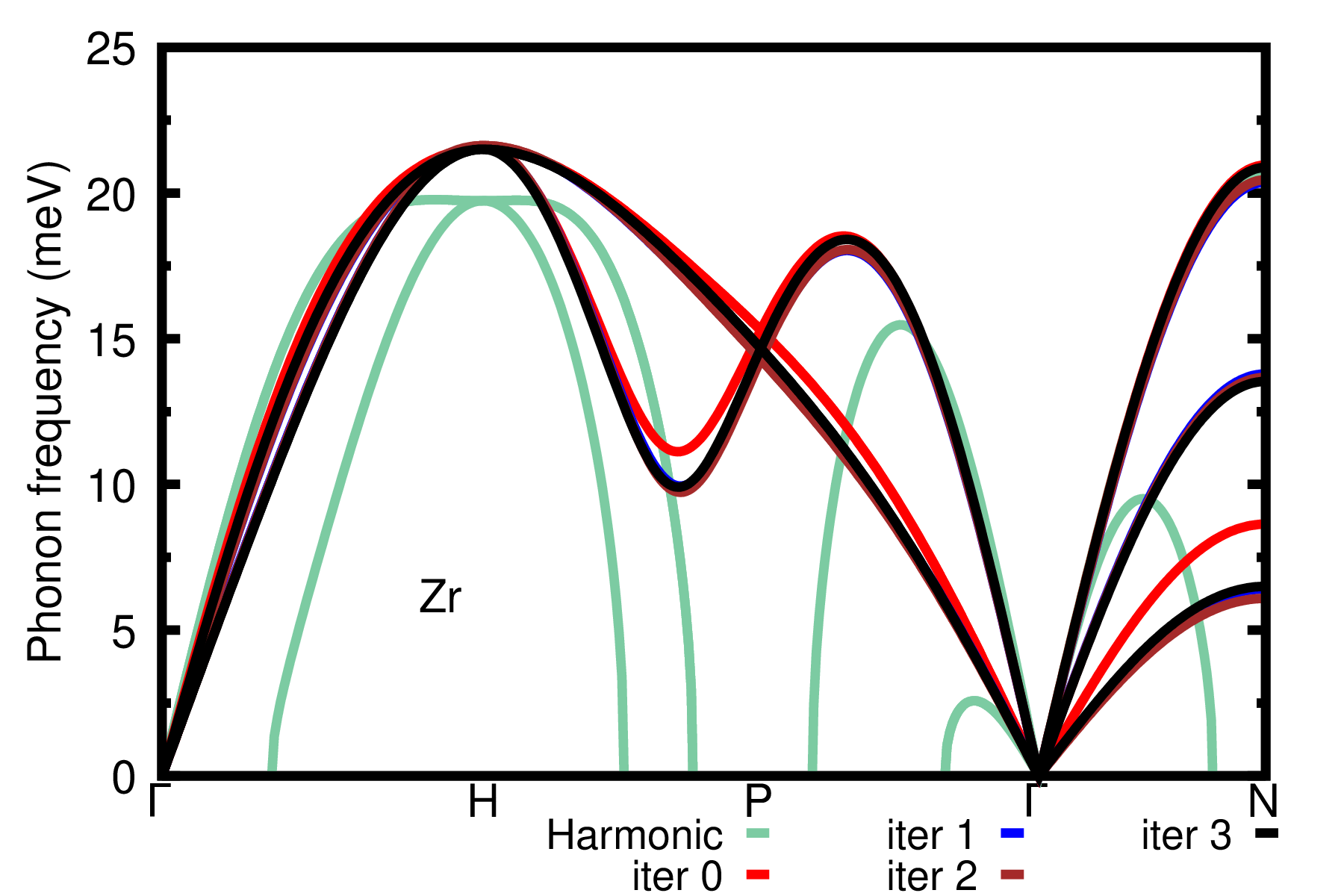
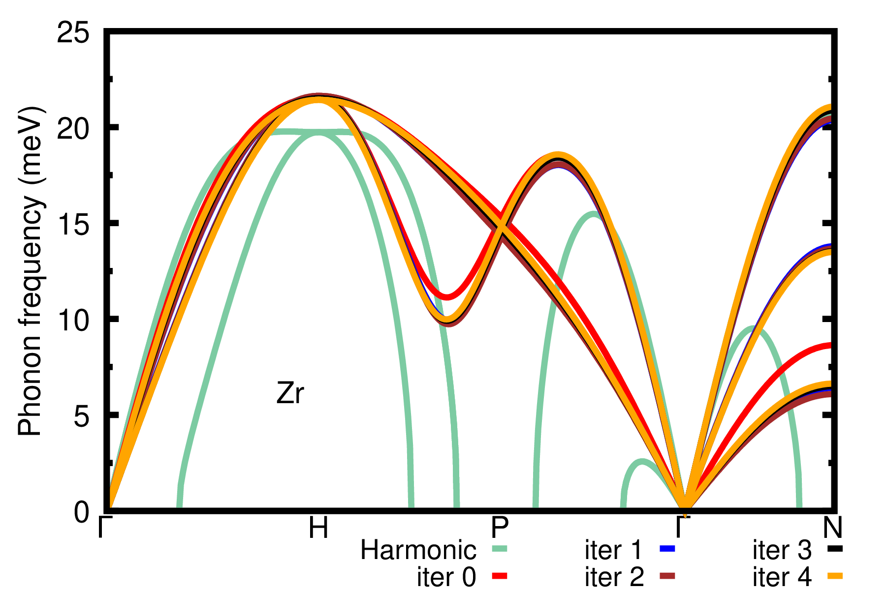
We can readily see that convergence is obtained at the third iteration; note that the result from the first iteration is still in excellent agreement with the converged result.
As a homework, also calculate the phonons of Zr at \(T=1188\) K using \(3\times3\times3\) supercells. HINT: Start the ASDM procedure from the IFCs of Zr at \(T=1188\) K obtained at the third iteration with \(2\times2\times2\) supercells (i.e. using 1188.00K_iter_03.fc). The result is provided in the plot below.
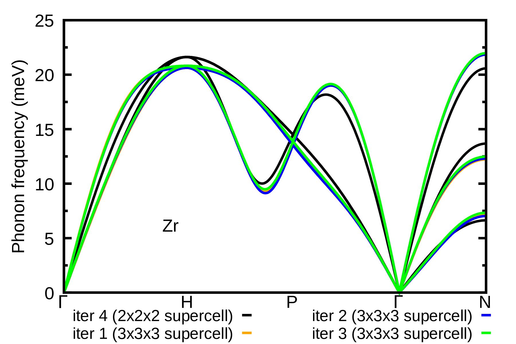
For the convergence of the phonon dispersion when larger supercells are used, please refer to the results in Ref. [Phys. Rev. B 108, 035155 (2023)]. Therein, results are obtained using more accurate settings, i.e. denser k-grid and higher kinetic energy cutoff.
To this end we also discuss four final important points:
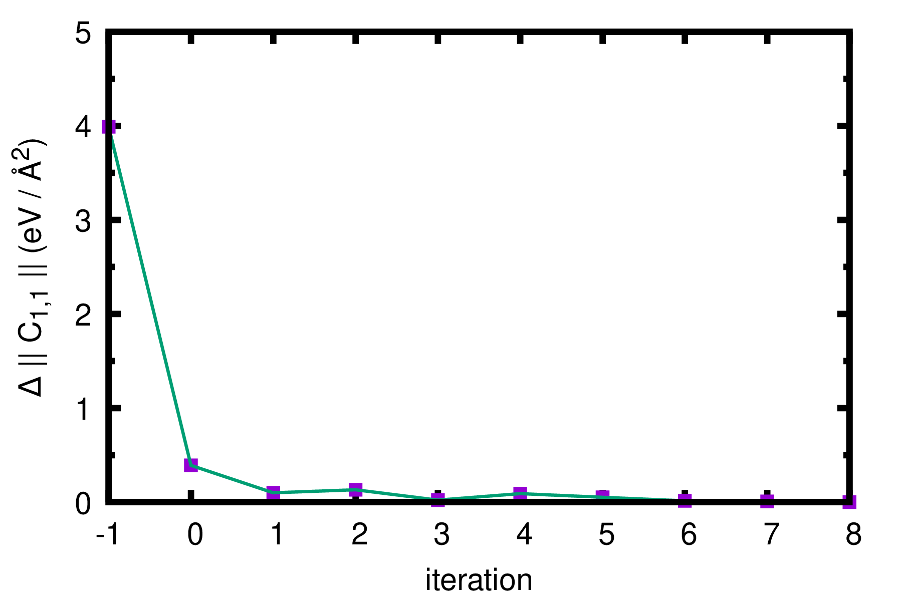
A quicker and more accurate way than checking the phonon dispersion is to plot the Frobenius norm (\(||.||\)) of the leading component of the IFCs matrix (\(\tilde{C}_{1 1 \alpha, 1 1 \alpha} (T)\)) as suggested in Ref. [Phys. Rev. B 84, 180301(R) (2011) ]. This information can be found by analysis of the first \(3\times3\) matrix in
FORCE_CONSTANTS_sym_1188.00K_iter_XX, where XX indicates the iteration. We note that convergence in IFCs guarantees essentially minimization of the system’s free energy. The result for a few more iterations is shown below. “iteration -1” corresponds to the harmonic \(||\tilde{C}_{1 1 \alpha, 1 1 \alpha}||\) and the difference is taken with respect to \(|| \tilde{C}_{1 1 \alpha, 1 1 \alpha} (T) ||\) of the last iteration. Note also that IFCs unit has been converted from Ry / Bohr \(^2\) to eV/Å \(^2\).
A full self-consistent phonon theory also minimizes the trial free energy with respect to nuclear coordinates. One can employ the Newton-Raphson method and find the nuclear coordinates for which \(\braket{\partial U / \partial \tau_{\kappa \alpha}}_T = 0\). This requires to solve self-consistently the equation \(\tau^{\rm new}_{p \kappa \alpha} (T) = \tau_{p \kappa \alpha} (T) + \tilde{C}^{-1}_{p \kappa \alpha, p \kappa \alpha} (T) \braket{F_{p \kappa \alpha}}_T\), using \(\tilde{C}_{p \kappa \alpha, p \kappa \alpha} (T)\) obtained at each iteration. In order to account for this feature in the ASDM we need to set the flag update_equil
= .true.when read_fd_forces= .true.. If we use this flag for the case of bcc Zr (point group symmetry \(m\bar3m\)), then the code will give \(\tau^{\rm new}_{p \kappa \alpha} (T) = \tau_{p \kappa \alpha} (T)\) (i.e. no change of the nuclear coordinates) at every iterative step. This comes as no surprise since symmetries are enforced and atoms in bcc Zr occupy only special Wyckoff positions. However, for systems containing atoms at general Wyckoff positions, update_equil= .true.will give new thermal equilibrium positions at each temperature that contribute to the minimization of the free energy. See for example the case of hydride compounds explored in Ref. [Commun. Phys. 6, 298 (2023)].Obtaining the polymorphous structure is not a necessary step. We found that this is a very useful step for obtaining positive definite initial IFCs matrix for systems with a double well potential. If the harmonic approximation gives a positive definite initial IFCs matrix, then one could start the iterative procedure without obtaining the polymorphous network.
After computing temperature-dependent anharmonic phonons using the ASDM, one could then do a ZG calculation using the new configuration and evaluate anharmonic electron-phonon properties. See for example Exercise 2.
Exercise 2
In this exercise we will learn how to calculate temperature-dependent anharmonic phonons of PbTe using \(2\times2\times2\) ZG supercells and the ASDM. Unlike Zr, seen in Exercise 1, PbTe is a polar material and a correction to the dynamical matrix arising from long-range dipole-dipole interactions is essential. Since the ASDM relies on the computation of IFCs by finite differences, we employ the mixed space approach described in Ref. [J. Phys. Condens. Matter 22 202201 (2010)], as implemented in matdyn.x. The key flags here to be used are fd = .true., na_ifc = .true., and incl_epsil = .true.. In this example, the harmonic IFCs matrix is positive definite and therefore the computation of the polymorphous structure is not required to initialize the ASDM procedure. Furthermore, here we will employ the anharmonic phonons to evaluate the band gap renormalization of PbTe.
Step 1
Go to the directory exercise2, create workdir, copy script.sh, and submit:
cd exercise2/; mkdir workdir; cd workdir
cp ../inputs/script.sh .
sbatch script.sh
The script will run scf and DFPT phonon calculations to obtain the (stable) harmonic phonons, and then start the ASDM procedure to evaluate anharmonic phonons at 300 K. The ASDM is performed for three iterations. The commands and workflow in the submission script script.sh are provided in this link.
The files scf.in, ph.in, q2r.in, and matdyn.in are provided here:
scf.in
&control
   calculation='scf'
   restart_mode='from_scratch'
   prefix = 'scf'
   outdir='./'
   pseudo_dir='./'
   tstress=.true.
   tprnfor=.true.
/
&system
   ibrav=2
   space_group = 225
   nat=2
   ntyp=2
   ecutwfc= 50
   A = 6.4440
/
&electrons
   diagonalization='david'
   mixing_mode='plain'
   mixing_beta=0.7
   conv_thr=1e-7
/
ATOMIC_SPECIES
  Pb 207.2 Pb.upf
  Te 127.60 Te.upf
K_POINTS {automatic}
  6 6 6 0 0 0
ATOMIC_POSITIONS (crystal_sg)
    Pb  4b
    Te  4a
Note: Here we provide the space group of the crystal, as given in the International Tables of Crystallography A (ITA), and the atomic coordinates in Wyckoff positions. This is an alternative way to specify the geometry of the system in Quantum Espresso which ensures that the symmetry of the crystal is respected.
ph.in
 &inputph
 prefix = 'scf',
 amass(1) = 207.2
 amass(2) = 127.60
 outdir = './'
 verbosity = 'high'
 ldisp = .true.
 fildyn = 'PbTe.dyn'
 tr2_ph = 1.0d-14
 nq1 = 2
 nq2 = 2
 nq3 = 2
/
q2r.in
&input
 fildyn='PbTe.dyn', zasr='crystal', flfrc = 'PbTe.222.fc'
/
matdyn.in
&input
 asr='all',
 flfrc='PbTe.222.fc', fldyn=' ', flfrq='PbTe_harm.freq',
 fleig=' ', q_in_cryst_coord = .true., q_in_band_form = .true.
/
3
0 0.5 0.5 100
0 0.0 0.0 100
0 0.5 0.5 100
We also note that the calculations are performed with unconverged settings (e.g. cutoff and k-point grid). To speed up the ASDM process, the script uses calculated output scf files given in folder fd_forces. ZG.x applies mixing of IFCs between iterations (mixing = .true.) and includes information of the Born effective charges and dielectric constant (incl_epsil = .true.) computed by DFPT. See for example files ZG_4.in and ZG_6.in.
Step 2
Type the following command to see the important files generated.
ls -lrt *freq *fc
PbTe.222.fc
PbTe_harm.freq
PbTe_300.00K_01.freq
300.00K_iter_01.fc
PbTe_300.00K_02.freq
300.00K_iter_02.fc
PbTe_300.00K_03.freq
300.00K_iter_03.fc
Those are the files containing the harmonic IFCs, ASDM IFCs, and the corresponding phonon frequencies. The indices 01, 02, 03 indicate the ASDM iteration.
Step 3
Now use plotband.x to obtain the data for the phonon dispersions as xmgr files, i.e.:
$QE/plotband.x
Input file > PbTe_harm.freq
Reading    6 bands at    201 k-points
Range:    0.0000  102.6916eV  Emin, Emax, [firstk, lastk] > 0 110
high-symmetry point:  0.0000 1.0000 0.0000   x coordinate   0.0000
high-symmetry point:  0.0000 0.0000 0.0000   x coordinate   1.0000
high-symmetry point:  0.0000 1.0000 0.0000   x coordinate   2.0000
output file (gnuplot/xmgr) > PbTe_harm.xmgr
bands in gnuplot/xmgr format written to file PbTe_harm.xmgr
output file (ps) >
stopping ...
Note: We use the name PbTe_harm.xmgr for the harmonic case, and the names iter_01.xmgr, iter_02.xmgr, and iter_03.xmgr for anharmonic phonon dispersions.
Step 4
Now plot the phonon dispersions using:
gnuplot gp_coms_iters.p
evince PbTe_300K_iters_ph_dispersion.pdf
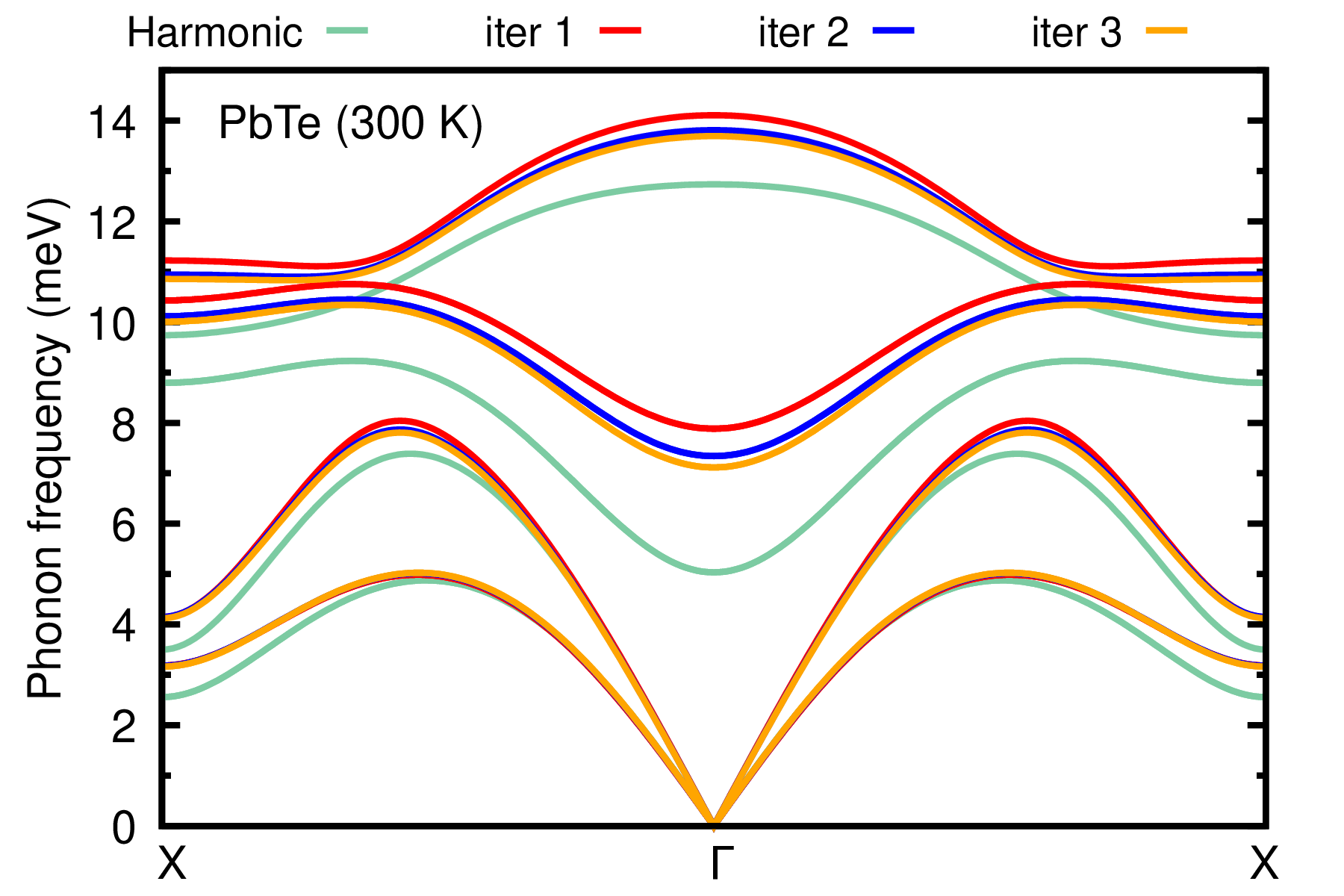
The ASDM is almost converged at the third iteration. If higher cutoff and denser k-grids are used, convergence can be achieved even at an earlier iteration.
Step 5
Now calculate the anharmonic phonon dispersion at 500 K using the script script_ASDM.sh. The submission script is provided in this link.
sbatch script_ASDM.sh
Step 6
Repeat the calculation but now for 700 K by changing T in the submission script script_ASDM.sh.
Step 7
Now obtain 500K_iter_01.xmgr and 700K_iter_01.xmgr from PbTe_500.00K_01.freq and PbTe_700.00K_01.freq using plotband.x (as above) and plot the phonon dispersions:
gnuplot gp_coms_T.p
evince PbTe_T_ph_dispersion.pdf
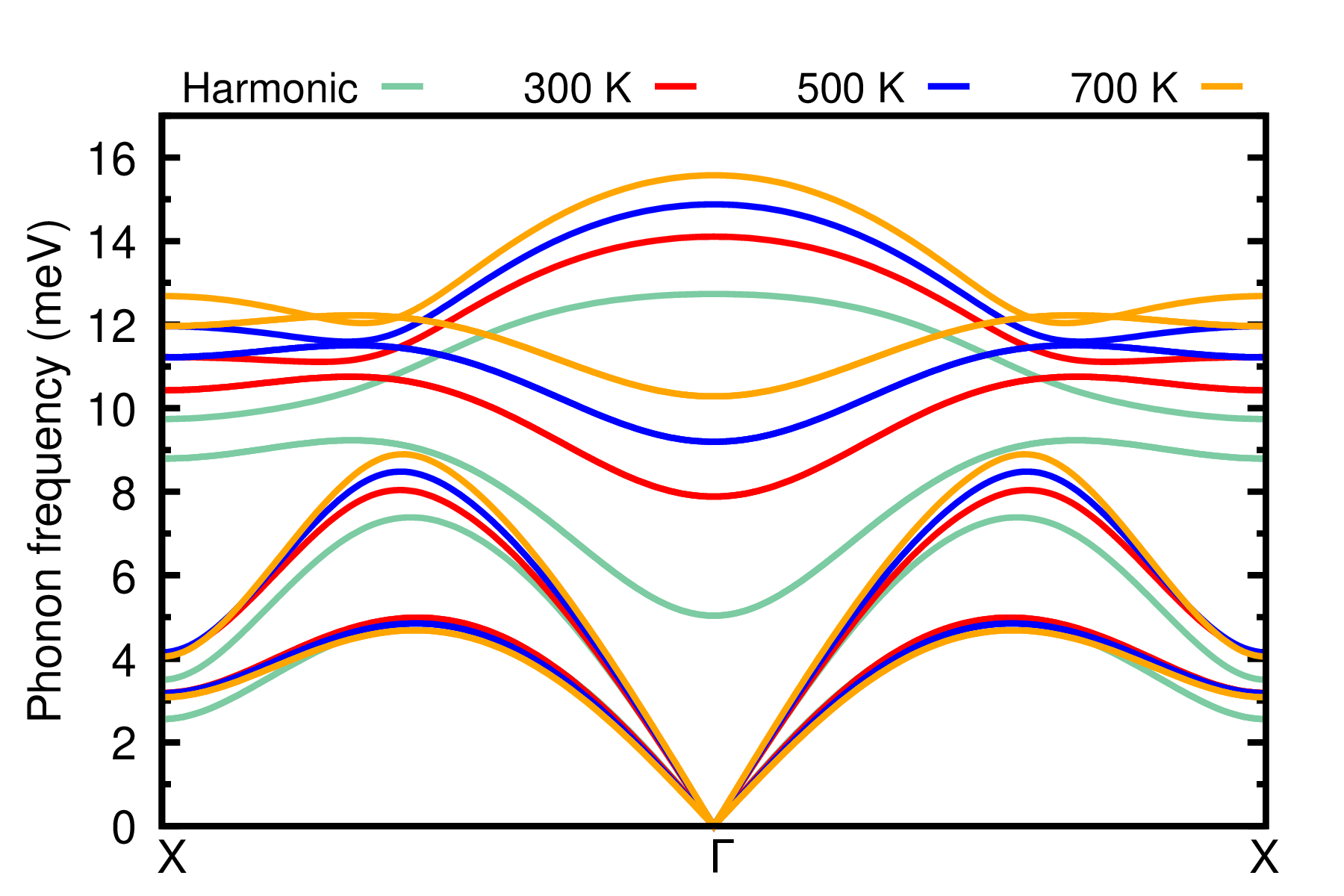
It is evident that anharmonicity is important to describe lattice dynamics in PbTe at elevated temperatures, particularly for the optical modes. Therefore, anharmonicity cannot be neglected in the description of electron-phonon properties in this system. In the following, we are going to calculate the phonon-induced band gap renormalization using anharmonic phonons and compare the result with the one obtained within the harmonic approximation.
Step 8
Submit the script script_harm.sh to evaluate the direct band gap of PbTe within the harmonic approximation at 300, 500, and 700 K using \(2\times2\times2\) ZG configurations. The script runs (i) a ZG.x calculation to generate the scf files, (ii) scf calculations for the equilibrium and T-dependent structures, and (iii) nscf calculations with empty bands for the equilibrium and T-dependent structures. The submission script is provided in this link.
sbatch script_harm.sh
The ZG file used (ZG_harm.in) is as shown below:
ZG_harm.in
&input
   asr='all',
   flscf = 'scf.in'
   flfrc='PbTe.222.fc'
   atm_zg(1) = 'Pb',
   atm_zg(2) = 'Te',
   T_array(1) = 300,
   T_array(2) = 500,
   T_array(3) = 700,
   dim1 = 2, dim2 = 2, dim3 = 2, incl_qA = .true.,
   synch = .true.
/
Note: PbTe.222.fc contains the harmonic IFCs. T_array(i) allows ZG configurations for multiple temperatures using the same set of signs generated by ZG.x.
The calculations should take around 3 minutes. While the calculations are running, let us discuss some aspects about the choice of the K-point (0.00 0.00 0.00) made in Kpoints.txt for the nscf calculation. The direct gap of cubic PbTe lies at the L-point (1/2, 1/2, 1/2) of the fundamental Brillouin zone (see Materials Project). Therefore, using a \(2\times2\times2\) supercell, the bands at the L-point are folded at the \(\Gamma\)-point of the supercell’s Brillouin zone. Note that this is not the case for other supercell sizes, e.g. \(3\times3\times3\), and therefore a different K-point should be chosen.
Step 9
Extract the band gap of the structure at static equilibrium and at finite temperatures using:
grep highest equil-nscf_222.out > tmp
awk '{print $8-$7}' tmp > equil_gap.dat
cat equil_gap.dat
0.6543
./gap_222.sh # script to obtain T-dependent gaps
cp gap_222_T.dat gap_222_T_harm.dat
cat gap_222_T_harm.dat
#  T (K)  E (eV)
   300    0.8999
   500    0.99453
   700    1.06219
The script gap_222.sh employs basic Linux commands to find the direct band gap of PbTe using the bands energy information printed in ZG-nscf_222_T.00K.out files. It takes the average of the four valence bands higher in energy and the four conduction bands lower in energy which are degenerate for the equilibrium structure. The degeneracy splitting is an artifact due to finite supercell size effects, as discussed in SDM: Exercise 1. The script gap_222.sh is provided in this link.
Step 10
Now submit the script script_anh.sh to evaluate the direct band gap of PbTe at 300, 500, and 700 K using \(2\times2\times2\) ZG supercells generated using anharmonic phonons. The script runs three ZG.x calculations to generate the scf files for each temperature using the corresponding T.00K_iter_01.fc files. Then it performs the scf calculations for the equilibrium and T-dependent structures, and nscf calculations with empty bands for the equilibrium and T-dependent structures. The submission script is provided in this link.
sbatch script_anh.sh
The calculations should take around 3 minutes. Here we provide the ZG_300K.in:
ZG_300K.in
&input
   asr='all',
   flscf = 'scf.in'
   flfrc='300.00K_iter_01.fc'
   atm_zg(1) = 'Pb',
   atm_zg(2) = 'Te',
   T = 300,
   dim1 = 2, dim2 = 2, dim3 = 2, incl_qA = .true.
   compute_error = .true., synch = .true., error_thresh = 0.4
   na_ifc = .true., fd =.true.
/
Note: Unlike file ZG_harm.in, here we provide only one temperature per ZG run since 300.00K_iter_01.fc corresponds to anharmonic phonons computed for 300 K. In addition, we add the flags fd = .true., na_ifc = .true. to account for long range effects since the IFCs in 300.00K_iter_01.fc are computed by finite differences. For the same reason, the flags fd = .true. and na_ifc = .true. are used in matdyn_0X.in (X = 01, 02, 03), ZG_X.in (X = 3, 4, 5, 6), and ZG_XK.in (X = 300, 400, 500). This is not the case for file ZG_harm.in, since initial harmonic IFCs (PbTe.222.fc) are computed by DFPT.
Step 11
Extract the direct band gap of PbTe at finite temperatures and compare it with the harmonic case using:
./gap_222.sh # script to obtain T-dependent gaps
cat gap_222_T.dat
#  T (K)  E (eV)
   300    0.84392
   500    0.86571
   700    0.92958
gnuplot gp_coms_gap.p; evince PbTe_Renormalization_T.pdf
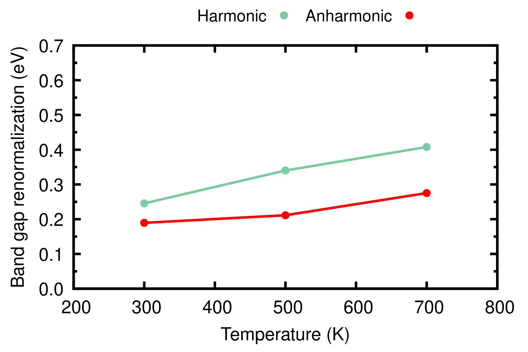
Here we show the band gap renormalization, i.e. we subtract the band gap at static equilibrium (0.654 eV) from the temperature-dependent band gap. At variance with conventional semiconductors, e.g. silicon and diamond, the direct band gap of PbTe increases with temperature which is consistent with exprimental measurements (see Ref. [Appl. Phys. Lett. 103, 262109 (2013)]). With these tutorial settings, anharmonicity leads to a correction of 30%-50% to the band gap renormalization. More accurate values can be obtained using larger ZG supercells, larger cutoff, denser grids, and inclusion of spin-orbit coupling.
Exercise 3
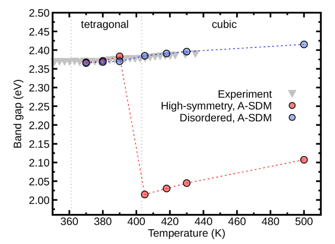
In this exercise we will explore anharmonic electron-phonon coupling in cubic CsPbBr\(_3\) (inorganic metal halide perovskite) by calculating the band gap renormalization, following Ref. [npj Comput. Mater. 9, 153 (2023)]. Here, anharmonic phonons are calculated by the ASDM and used to generate ZG displacements for the monomorphous (high-symmetry) and ground state polymorphous (low-symmetry) structures in \(2\times2\times2\) supercells. The difference in the computed band gap renormalization for the two cases is strikking, showing that polymorphism (or local disorder) plays a key role in predicting accurately electron-phonon properties in cubic perovskites.
Step 1
Go to exercise3, create workdir, copy script.sh from inputs, and submit:
cd exercise3/; mkdir workdir; cd workdir
cp ../inputs/script.sh .
sbatch script.sh
Note: ZG.x applies mixing of IFCs between iterations (mixing = .true.) and includes information of the Born effective charges and dielectric constant (incl_epsil = .true.) computed by DFPT at the initial step. In addition, we use the flags fd = .true., na_ifc = .true. to account for long range effects since the IFCs at each iteration are computed by finite differences. See for example files ZG_5.in and ZG_7.in.
The script will run scf and DFPT phonon calculations to obtain the harmonic (unstable) phonons, and then start the ASDM approach to evaluate anharmonic phonons at 450 K. The ASDM is performed for (i) the zeroth iteration to obtain the polymorphous structure and its stable phonons and (ii) for the first and second iterations to obtain self-consistent anharmonic phonons. The commands and workflow in the submission script script.sh are provided in this link. To speed up the ASDM, the script uses calculated output scf files given in fd_forces directory. The script should take around 4 minutes to finish.
The files scf.in, ph.in, q2r.in, matdyn.in are provided here:
scf.in
&control
        calculation='scf'
        restart_mode='from_scratch'
        prefix = 'scf'
        outdir='./'
        pseudo_dir='./'
        tstress=.true., tprnfor=.true.
/
&system
        ibrav=1, A = 5.874, nat=5, ntyp=3,
        ecutwfc=  40
/
&electrons
        diagonalization='david'
        mixing_mode='plain'
        mixing_beta=0.7, conv_thr=1e-6
/
ATOMIC_SPECIES
Cs 132.90545 Cs.upf
Pb 207.2  Pb.upf
Br 79.904 Br.upf
K_POINTS {automatic}
4 4 4 0 0 0
ATOMIC_POSITIONS (crystal)
 Cs  0.500000 0.500000 0.500000
 Pb  0.000000 0.000000 0.000000
 Br  0.000000 0.000000 0.500000
 Br  0.000000 0.500000 0.000000
 Br  0.500000 0.000000 0.000000
ph.in
&inputph
   prefix = 'scf'
   outdir = './'
   fildyn = 'CsPbBr3.dyn'
   tr2_ph = 1.0d-12
   ldisp = .true.
   nq1 = 2, nq2 = 2, nq3 = 2
/
q2r.in
&input
 fildyn='CsPbBr3.dyn', flfrc = 'CsPbBr3.222.fc'
/
matdyn.in
&input
    asr='all',
    flfrc='CsPbBr3.222.fc', fldyn='CsPbBr3.dyn.mat', flfrq='CsPbBr3.freq',
    fleig='CsPbBr3.dyn.eig', q_in_cryst_coord = .true., q_in_band_form = .true.
/
5
0.0000    0.5000    0.000000  100
0.5000    0.5000    0.500000  100
0.5000    0.5000    0.000000  100
0.0000    0.0000    0.000000  100
0.5000    0.5000    0.500000  1
Step 2
Type the following command to see the important files generated.
ls -lrt *freq *fc
CsPbBr3.222.fc # harmonic
CsPbBr3.freq   # harmonic
poly_iter_00.fc
CsPbBr3_poly.freq
450.00K_iter_01.fc
CsPbBr3_01.freq
450.00K_iter_02.fc
CsPbBr3_02.freq
Those are the files containing the harmonic IFCs, ASDM IFCs, and corresponding phonon frequencies. The indices 00, 01, 02 indicate the ASDM iteration, with index 00 representing the 0th iteration for the polymorphous structure.
Step 3
Now use plotband.x to obtain the data for the phonon dispersions as xmgr files, e.g.:
$QE/plotband.x
Input file > CsPbBr3.freq
Reading   15 bands at    401 k-points
Range:  -45.5651  176.0997eV  Emin, Emax, [firstk, lastk] > -50 180
high-symmetry point:  0.0000 0.5000 0.0000   x coordinate   0.0000
high-symmetry point:  0.5000 0.5000 0.5000   x coordinate   0.7071
...
high-symmetry point:  0.5000 0.5000 0.5000   x coordinate   2.7802
output file (gnuplot/xmgr) > CsPbBr3_harm.xmgr
bands in gnuplot/xmgr format written to file CsPbBr3_harm.xmgr
Note: Use the name CsPbBr3_harm.xmgr for the harmonic monomorphous case, CsPbBr3_poly.xmgr for the polymorphous case, and iter_01.xmgr and iter_02.xmgr for the ASDM phonon dispersions up to iteration 2.
Step 4
Plot the phonon dispersions using:
cp ../inputs/gp_coms_iters.p .
gnuplot gp_coms_iters.p
evince CsPbBr3_450K_iters_ph_dispersion.pdf
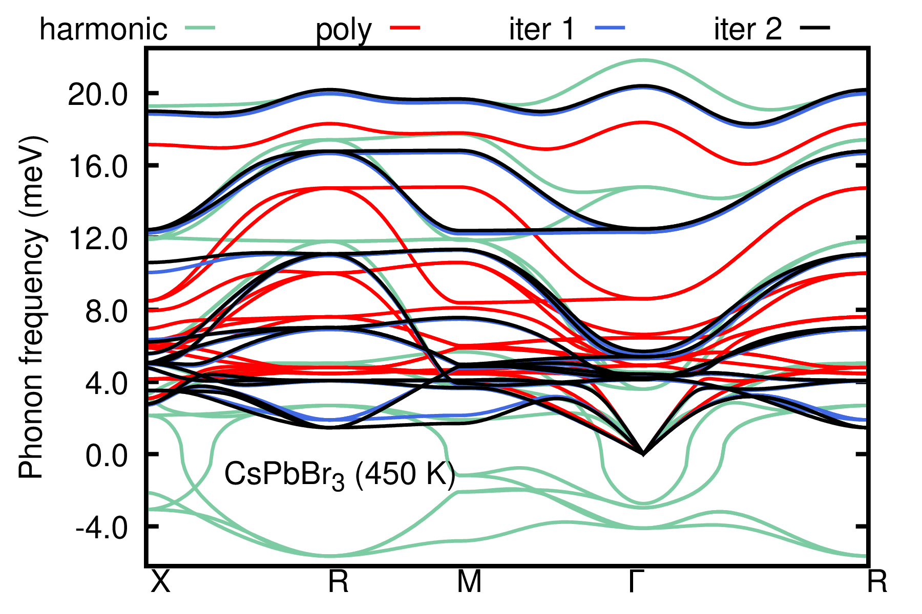
The harmonic phonons computed for the monomorphous structure (green) exhibit large instabilities. The computed symmetrized phonons for the polymorphous structure are stable (red), and corrections to the real part of the phonon self-energy are included via the ASDM (blue and black). The ASDM is almost converged at the second iteration. Please refer to Ref. [Phys. Rev. B 108, 035155 (2023)] for converged settings and results.
Step 5
Calculate the band gap renormalization of the monomorphous structure at 430, 450, 470, and 500 K
using the ASDM phonons.
cp ../inputs/script_mono_gap.sh .
sbatch script_mono_gap.sh
The commands in script_mono_gap.sh are provided in this link. The ZG files are generated using the anharmonic IFCs in 450.00K_iter_02.fc via the input ZG_multi_T.in:
ZG_multi_T.in
&input
   asr='all', flfrc='450.00K_iter_02.fc'
   flscf = 'scf.in'
   T_array(1) = 430, T_array(2) = 450, T_array(3) = 470, T_array(4) = 500
   atm_zg(1) = 'Cs', atm_zg(2) = 'Pb',  atm_zg(3) = 'Br'
   dim1 = 2, dim2 =2, dim3 =2, incl_qA = .true.
   synch = .true.,
   na_ifc = .true., fd = .true.
/
Note: For maximum accuracy, one should evaluate the ASDM phonons for each temperature separately. Here, we assume that phonons from 430 to 500 K do not change significantly.
The script script_mono_gap.sh (i) runs scf calculations for the static-equilibrium and ZG configurations of the monomorphous structure, (ii) prepares nscf files via script mono.sh provided in this link, and (iii) runs nscf calculations at \(\Gamma\) point to obtain information of the band energies for filled and empty bands. We choose \(\Gamma\) point since the band gap of CsPbBr\(_3\) is at the R point (1/2 1/2 1/2) of the fundamental Brillouin zone, and thus folded at the center of the Brillouin zone of a \(2\times2\times2\) supercell. All calculations should take around 7 minutes and 30 seconds.
Step 6
Extract the temperature-dependent band gap and renormalization from the nscf files using:
mono_gap=$(grep highest equil-nscf_222.out | awk '{print $8-$7}')
echo $mono_gap
1.4377
grep highest ZG-nscf_222_*.out > tmp
awk '{print $1, $8, $9, $9-$8, $9-$8-'$mono_gap'}' tmp > Renorm_mono_T.dat
sed -i 's/ZG-nscf_222_//g' Renorm_mono_T.dat
sed -i 's/K.out://g' Renorm_mono_T.dat
cat Renorm_mono_T.dat
#  T(K)    VBM(eV) CBM(eV)  Gap(eV)  Renorm. (eV)
  430.00   3.3770  5.2349   1.8579   0.4202
  450.00   3.3623  5.2357   1.8734   0.4357
  470.00   3.3479  5.2365   1.8886   0.4509
  500.00   3.3266  5.2374   1.9108   0.4731
Step 7
Calculate the band gap renormalization at 430, 450, 470, and 500 K using the ASDM phonons but now displace
the atoms of the polymorphous network.
cp ../inputs/script_poly_gap.sh .
sbatch script_poly_gap.sh
The commands in script_poly_gap.sh are provided in this link. The script (i) prepares scf and nscf files via the script poly.sh which is provided in this link. The displacements (see files displ_TK.txt) are obtained by taking the difference between the ZG and high-symmetry coordinates. Then, the displacements are added on the coordinates of the polymorphous structure. The script also (ii) runs scf calculations for the static-equilibrium and ZG configurations of the polymorphous structure, and (iii) runs the correspondng nscf calculations to obtain information of the band energies for filled and empty bands. All calculations should take around 7 minutes and 30 seconds.
Step 8
Extract the temperature-dependent band gap and renormalization from the nscf files using:
poly_gap=$(grep highest ZG-nscf_poly_iter_00.out | awk '{print $8-$7}')
echo $poly_gap
2.0189
grep highest ZG-nscf_poly_*K.out > tmp
awk '{print $1, $8, $9, $9-$8, $9-$8-'$poly_gap'}' tmp > Renorm_poly_T.dat
sed -i 's/ZG-nscf_poly_//g' Renorm_poly_T.dat
sed -i 's/K.out://g' Renorm_poly_T.dat
cat Renorm_poly_T.dat
#  T(K)    VBM(eV) CBM(eV)  Gap(eV)  Renorm. (eV)
  430.00   2.9337  5.1302   2.1965   0.1776
  450.00   2.9274  5.1285   2.2011   0.1822
  470.00   2.9213  5.1266   2.2053   0.1864
  500.00   2.9121  5.1235   2.2114   0.1925
Can you compare first the band gap of the monomorphous and polymorphous structures without the effect of electron-phonon coupling? Polymorphism induces a band gap opening of 0.58 eV in good agreement with the value reported in Table 1 of Ref. [npj Comput. Mater. 9, 153 (2023)]. Furthermore, the band gap renormalization calculated for the monomorphous and polymorphous structures at 430 K is 420 meV and 178 meV, respectively. These values are in fair agreement with those reported in Ref. [npj Comput. Mater. 9, 153 (2023)], showing the significant effect of polymorphism on electron-phonon coupling in halide perovskites. Note that here we use a small supercell size and do not include the effect of spin-orbit coupling, which are important for obtaining more accurate results.
Step 9
Plot the band gap renormalization for the monomorphous and polymorphous networks:
cp ../inputs/gp_coms_gap.p .
gnuplot gp_coms_gap.p
evince CsPbBr3_renormalization.pdf
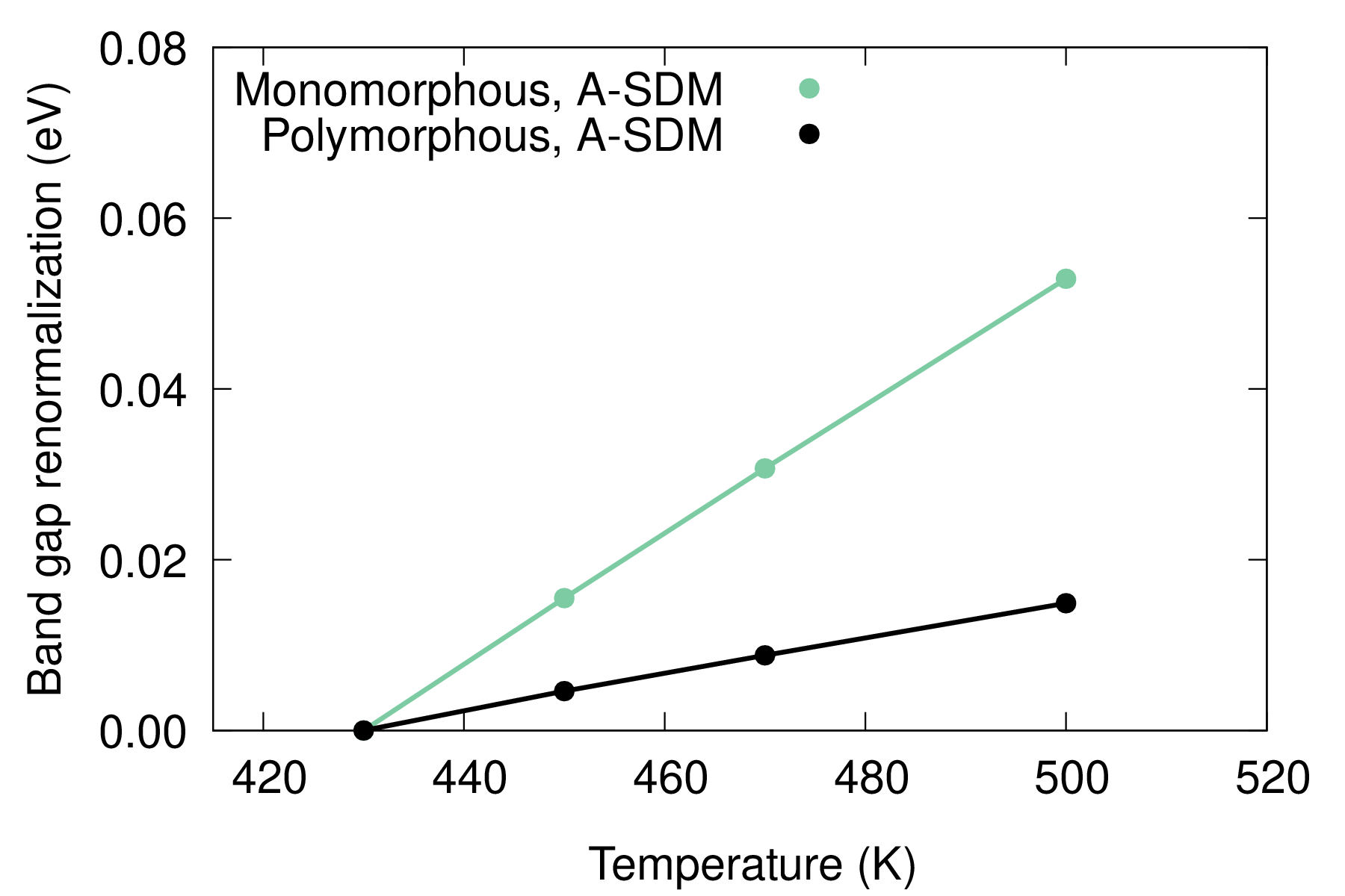
To facilitate comparison, we show the band gap renormalization with respect to the gap at 430 K. The band gap of the polymorphous structure increases much slower with temperature than the one calculated for the monomorphous structure. Evaluating electron-phonon renormalization using the polymorphous structure is crucial for explaining experimental data, especially across phase transitions, as shown in Figure 6 of Ref. [npj Comput. Mater. 9, 153 (2023)], which is reproduced below.
The success of the polymorphous network is related to the fact that electrons will mostly see the nuclei in the infinitely more stable polymorphous configurations that exist energetically. Can you extract the energy lowering of the polymorphous structure (ZG-scf_poly_iter_00.out) with respect to the monomorphous structure (equil-scf_222.out)? As homework, you can restart the calculations by setting a different initial temperature in files ZG_X.in (X = 1, 2, 3). This will generate different coordinates for the polymorphous structure (but very similar ground state energy). Moreover, the final results obtained in this tutorial should not be affected significantly.