Special displacement method
04/08/2026
Note
Hands-on based on QE-v7.3.1 and EPW-v5.9
Note
It is perfectly reasonable to obtain ZG displacements that differ from those reported in this tutorial. These differences arise from numerical accuracy in the phonon calculations and from the gauge freedom of the vibrational modes: modes obtained by diagonalizing the dynamical matrix may differ by a phase factor (or by a unitary transformation in the case of degeneracy) when computed on different HPC systems. The final results, within reasonable accuracy, are not affected by these differences.
In this tutorial we will learn to use the core capabilities of the ZG.x code for applying the special displacement method (SDM) and how to combine it with standard Density Functional Theory (DFT) calculations for evaluating temperature-dependent properties.
Prerequisites
This tutorial assumes that Quantum ESPRESSO and EPW have already been downloaded and compiled.
If you have not yet completed these steps,
please follow the Installation and setup tutorial before continuing.
The examples below also assume that the environment variables used to run the executables
(such as $QE, $RUN_PW, and $RUN_ZG) have been defined as described in the Installation and setup .
Note that variables defined with export only apply to the current terminal session.
If you compiled the code previously but are starting a new session,
you may need to redefine the run variables following the instructions in Defining run commands.
If the setup tutorial has been followed in the current session, the commands below should work directly in your terminal.
Download input files
Download the tutorial tarball (tutorial02.tar.gz) from this link and untar.
You are advised to prepare the following script file, e.g. script.sh:
#!/bin/bash
#SBATCH --job=SDM
#SBATCH --nodes=1
#SBATCH --ntasks-per-node=48
#SBATCH --time=01:00:00
#SBATCH --account=
#SBATCH --partition=
#SBATCH --reservation=
# Load Modules
#
QE=/path_to/q-e/bin # path to "bin" of q-e
export RUN_PW="mpirun -np 4 $QE/pw.x"
export RUN_PH="mpirun -np 4 $QE/ph.x"
export RUN_Q2R="$QE/q2r.x"
export RUN_MATDYN="$QE/matdyn.x"
export RUN_ZG="$QE/ZG.x"

cd $PWD
For each calculation, pass the command at the bottom of the script and submit the job, e.g. sbatch script.sh. Also set the following environment variable in your shell:
export QE=/path_to/q-e/bin/
All necessary executables and the ZG module are compiled with EPW, i.e. with make epw. To use local executables go to q-e/EPW/ZG/src/local and type ./compile_ifort.sh. The description of all input flags is available in this link .
Exercise 1: Generation of the ZG configuration and DFT-ZG calculation (silicon)
Exercise 2: Temperature-dependent band structures (silicon)
Exercise 3: Temperature-dependent optical spectra (silicon)
Exercise 4: Band gap renormalization for various temperatures (diamond)
Exercise 5: Multiphonon diffuse scattering (graphene)
Exercise 6: Phonon unfolding (P-doped silicon)
Exercise 1
In this exercise we will generate the ZG configuration of silicon in a \(3\times3\times3\) supercell for the temperature \(T = 0\) K and run a DFT-ZG calculation. In the following, all steps for obtaining the phonons and interatomic force constants (IFCs) of silicon are provided; but to speed up the process you can skip the first four steps.
Note: in this tutorial we show how to obtain all input and output files. The directories inputs and outputs are used as a reference or to speed up the process. Most of the temperature-dependent calculations will be performed for \(T = 0\) K; one can repeat the steps using a different temperature.
Untar the tarbal and go to directory exercise1, and create directory workdir:
cd $SCRATCH
tar -xvf tutorial02.tar.gz; cd tutorial02/exercise1; mkdir workdir
Note: For generating successfully a ZG configuration you need to make sure that the phonon dispersion is as you would expect (compare with literature). If there exist modes with negative frequencies, the code excludes them. If the system is anharmonic one should consider to evaluate anharmonic phonons using the ASDM (see ASDM: Exercise 1) ; see next tutorial.
Step 1
Run a self-consistent calculation for silicon in the workdir.
Note: The energy cutoff ecutwfc needed for convergence should be 30 Ry. One can also try different pseudos, see for example Pseudo Dojo library.
cd workdir; cp ../inputs/si.scf.in .; cp ../inputs/Si.pz-vbc.UPF .
$RUN_PW -nk 4 < si.scf.in > si.scf.out
Step 2
Run a ph.x calculation on a homogeneous \(4\times4\times4\) \(\mathbf{q}\)-point grid using the input:
si.ph.in
&inputph
   amass(1) = 28.0855,
   prefix   = 'si'
   outdir   = './'
   ldisp    = .true.
   fildyn   = 'si.dyn'
   tr2_ph   = 1.0d-12
   nq1      = 4, nq2 = 4, nq3 = 4
/
cp ../inputs/si.ph.in .
$RUN_PH -nk 4 < si.ph.in > si.ph.out
This will generate 8 si.dynX output files containing the dynamical matrix calculated for each irreducible \(\mathbf{q}\)-point. The list of irreducible \(\mathbf{q}\)-points is written in the si.dyn0 file.
Step 3
Run a q2r.x calculation to obtain the interatomic force constants (IFC)
file using the input:
q2r.in
&input
 fildyn='si.dyn', flfrc = 'si.444.fc'
/
cp ../inputs/q2r.in .
$RUN_Q2R < q2r.in > q2r.out
This will generate si.444.fc which contains the IFCs.
Step 4
Run a matdyn.x calculation to check the phonon dispersion:
matdyn.in
&input
    asr='all', amass(1)=28.0855,
    flfrc='si.444.fc', fldyn='si.dyn.mat', flfrq='si.freq', fleig='si.dyn.eig',
    q_in_cryst_coord = .false., q_in_band_form = .true.
/
 9
 0.00  0.00  0.00  100
 0.75  0.75  0.00  1
 0.25  1.00  0.25  100
 0.00  1.00  0.00  100
 0.00  0.00  0.00  100
 0.50  0.50  0.50  100
 0.00  1.00  0.00  100
 0.50  1.00  0.00  100
 0.50  0.50  0.50  100
cp ../inputs/matdyn.in .
$RUN_MATDYN < matdyn.in > matdyn.out
$QE/plotband.x
Input file > si.freq
Reading    6 bands at    702 k-points
Range:    0.0000  510.0194eV  Emin, Emax, [firstk, lastk] > 0 600
high-symmetry point:  0.0000 0.0000 0.0000   x coordinate   0.0000
high-symmetry point:  0.7500 0.7500 0.0000   x coordinate   1.0607
...
high-symmetry point:  0.5000 0.5000 0.5000   x coordinate   5.3534
output file (gnuplot/xmgr) > si_ph_dispersion.xmgr
bands in gnuplot/xmgr format written to file si_ph_dispersion.xmgr

output file (ps) >
stopping ...
matdyn.x will generate si.freq which contains the phonon frequencies along the specified path in the Brillouin zone. Then we combine si.freq with plotband.x to obtain si_ph_dispersion.xmgr in gnuplot/xmgr format for the phonon dispersion. To plot the phonon dispersion type:
cp si_ph_dispersion.xmgr ../gnuplot/.
cd ../gnuplot/; gnuplot gp_coms.p; evince ph_dispersion_444.pdf
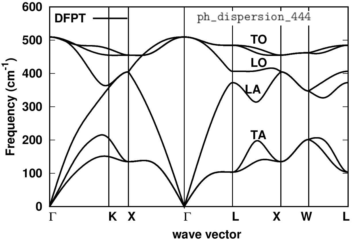
Is the phonon dispersion as you expect? One can verify the results with literature data. Once you have obtained the IFC file (e.g. here si.444.fc) and verified the correctness of your phonons, you are ready to perform a ZG.x calculation.
Optional: If you have skipped the four steps above, you can copy the IFC file from inputs into workdir:
cd ../workdir; cp ../inputs/si.444.fc .
Step 5
Run a ZG calculation using the input:
ZG_333.in
&input
    flfrc='si.444.fc',
    asr='all', amass(1)=28.0855, atm_zg(1) = 'Si',
    flscf = 'si.scf.in'
    T = 0.00,
    dim1 = 3, dim2 = 3, dim3 = 3
    compute_error = .true., synch = .true., error_thresh = 0.1, niters = 15000
    incl_qA = .false.
/
Note: The \(\mathbf{q}\)-point grid (nq1\(\times\) nq2\(\times\) nq3) used to obtain the dynamical matrices should not be necessarily the same with the supercell size (dim1\(\times\) dim2\(\times\) dim3). In particular, dimX is independent of nqX, since ZG.x takes advantage of Fourier interpolation as implemented in matdyn.x; thus any size of ZG configuration can be generated from si.444.fc.
cd ../workdir
cp ../inputs/ZG_333.in .
$RUN_ZG < ZG_333.in > ZG_333.out
The input format of ZG_333.in is similar to matdyn.in. Lines 2 and 3 contain input variables as in matdyn.in (note that a new feature for the acoustic sum rule, asr, is added with asr = 'all', it can also be simple or crystal); in line 4 we provide the name of the unit-cell scf file (flscf) used to calculate the phonons. The information therein is read to generate the corresponding supercell scf file. In lines 5 and 6 we provide the temperature (T) in Kelvin and supercell dimensions (dimX) for which ZG displacements are generated; line 7 contains all flags related to the error minimization (discussed later); in line 8 we specify whether we want to include, or not, \(\mathbf{q}\)-points in set \(\mathcal{A}\) using the flag incl_qA.
The output files from a ZG.x run are: (a) ZG-configuration_0.00K.dat and equil_pos.dat which contain the ZG (quantum nuclei at 0 K) and equilibrium (classical nuclei at 0 K) coordinates in angstroms, and (b) ZG-scf_333_0.00K.in and equil-scf_333.in which are the corresponding scf files for performing calculations in a \(3\times3\times3\) supercell.
Step 6
Run a self-consistent calculation for silicon with the nuclei clamped at their equilibrium and ZG coordinates (for \(T\) = 0.00 K) in the supercell.
mpirun -np 48 $QE/pw.x -nk 3 < equil-scf_333.in > equil-scf_333.out
mpirun -np 48 $QE/pw.x -nk 8 < ZG-scf_333_0.00K.in > ZG-scf_333_0.00K.out
Note: parallelization over 3 and 8 k-points.
The file equil-scf_333.in is also provided here:
equil-scf_333.in
&control
  calculation = 'scf'
  restart_mode = 'from_scratch'
  prefix = 'equil-si'
  pseudo_dir = './'
  outdir = './'
/
&system
  ibrav = 0
  nat =   54
  ntyp =    1
  ecutwfc =  20.00
  occupations = 'fixed'
  smearing = 'gaussian'
  degauss =   0.0D+00
/
&electrons
  diagonalization = 'david'
  mixing_mode= 'plain'
  mixing_beta = 0.70
  conv_thr =   0.1D-06
/
ATOMIC_SPECIES
   Si   28.085 Si.pz-vbc.UPF
K_POINTS automatic
   2   2   2   0   0   0
CELL_PARAMETERS {angstrom}
     -8.09641133      0.00000000      8.09641133
      0.00000000      8.09641133      8.09641133
     -8.09641133      8.09641133      0.00000000
ATOMIC_POSITIONS {angstrom}
   Si    0.00000000   0.00000000   0.00000000
   Si   -2.69880378   0.00000000   2.69880378
   Si   -5.39760755   0.00000000   5.39760755
...
Note: Cell parameters, number of atoms, k-grid, and atomic coordinates have been modified automatically based on the supercell dimensions. The code will always generate the lattice information in angstroms.
The file ZG-scf_333_0.00K.in is also provided here:
ZG-scf_333_0.00K.in
&control
  calculation = 'scf'
  restart_mode = 'from_scratch'
  prefix = 'ZG-0.00K-si'
  pseudo_dir = './'
  outdir = './'
/
&system
  ibrav = 0
  nat =   54
  ntyp =    1
  ecutwfc =  20.00
  occupations = 'fixed',  smearing = 'gaussian', degauss =   0.0D+00
/
&electrons
  diagonalization = 'david'
  mixing_mode= 'plain'
  mixing_beta = 0.70
  conv_thr =   0.1D-06
/
ATOMIC_SPECIES
   Si   28.085 Si.pz-vbc.UPF
K_POINTS automatic
   2   2   2   0   0   0
CELL_PARAMETERS {angstrom}
     -8.09641133      0.00000000      8.09641133
      0.00000000      8.09641133      8.09641133
     -8.09641133      8.09641133      0.00000000
ATOMIC_POSITIONS {angstrom}
...
Note: Same information with equil-scf_333.in, except for the prefix and atomic positions. In general, one should add no_sym = .true., since symmetries do not apply after ZG displacements. The information printed by the code for constructing these scf files is basic; so for more complex cases one can modify the files based on their calculation needs.
While the calculations are running, let us discuss some aspects about the generation of the ZG-configuration file. Type:
grep -3 "Optimum" ZG_333.out | tail -4
Optimum configuration found !

Sum of diagonal terms per q-point:    0.416464
Error and niter index:    0.044777       6
This information is printed during a ZG.x run when the optimum configuration is found. Line 3 gives the sum of all diagonal terms per q-point, representing the denominator of Eq. (54) in Ref. [Phys. Rev. Res. 2, 013357 (2020) ]. The first number in line 4 represents the value of the minimization function \(E(\{S_{{\bf q} \nu}\})\) given by Eq. (54) in Ref. [Phys. Rev. Res. 2, 013357 (2020) ]. The integer in line 4 represents the number of attempts required to achieve \(E(\{S_{{\bf q} \nu}\})\) smaller than the value specified for error_thresh. If this number exceeds the integer specified by niters flag, then ZG.x will stop without printing the ZG-configuration file. A general rule is: the larger the supercell, the fewer attempts are required to achieve \(E(\{S_{{\bf q} \nu}\})\) < error_thresh. The reason is: the order of choosing the unique set of signs, assigned to separate q-points, is less important as we approach the thermodynamic limit. Now type:
head -3 ZG-configuration_0.00K.dat
Temperature is:     0.00  K
Atomic positions          54
Si       0.12836811      0.00747083      0.06987595
Lines 1 and 2 give the temperature for which ZG displacements are generated and the total number of atomic coordinates. In line 3, we have the first ZG atomic coordinate. It is perfectly reasonable to find different ZG coordinates, since the modes obtained by diagonalizing the dynamical matrix can differ by a phase factor (or a unitary matrix in case of degeneracy) if the processor, or compiler, or libraries have changed. The eigenvalues should remain the same. The flag synch applies a smooth Berry connection and aligns the sign of the modes with respect to a reference mode, but the sign of this reference depends on the machine. Degeneracy is not taken into account. The best way to check the validity of your configuration is by comparing the anisotropic mean-squared displacement tensor with the exact values, both printed in ZG_333.out. To this aim type:
grep -15 "Anisotropic" ZG_333.out | tail -16
Anisotropic mean-squared displacement tensor vs exact values (Ang^2):

Atom: 1
-------
 ZG_conf:   Si    0.002583   0.002118   0.002354
   Exact:   Si    0.002339   0.002339   0.002339

Atom: 2
-------
 ZG_conf:   Si    0.002281   0.002400   0.002298
   Exact:   Si    0.002339   0.002339   0.002339


  off-diagonal terms
  Si   -0.000026  -0.000449  -0.000525
  Si    0.000395  -0.000460  -0.001429
Reducing error_thresh brings the anisotropic displacement tensor closer to the exact values. Note that in the previous versions of the code these values were multiplied by \(8\pi^2\). Now check whether the calculations have finished and type:
grep ! *scf_333*out
equil-scf_333.out:!    total energy              =    -427.83892822 Ry
ZG-scf_333_0.00K.out:!    total energy              =    -427.72146756 Ry
These are the total energies (Kohn-Sham potential energy) of the equilibrium and ZG structures. What is the difference between the two values and what is the reason of this difference? The difference is \(\Delta E_{\rm KS} = 0.1175\) Ry and is due to the vibrational potential energy. To check this type:
grep -5 "Potent" ZG_333.out
 Temperature is:     0.00  K
==============================================

 Total vibrational energy:    0.24054327 Ry at    0.00 K

         Potential energy:    0.12027163 Ry at    0.00 K

           Kinetic energy:    0.12027163 Ry at    0.00 K

  Vibrational free energy:    0.24054327 Ry at    0.00 K
Our computed \(\Delta E_{\rm KS}\) is indeed almost equal to half the total vibrational energy, since a DFT calculation will not account for the vibrational kinetic energy contribution. The value 0.117 Ry deviates from 0.120 Ry, since (i) we exclude from our calculations the q-points belonging in set \(\mathcal{A}\) and (ii) due to the error coming by using small ZG configurations. As we use larger supercells this small deviation reduces to zero and \(\Delta E_{\rm KS} =\) Total vibrational energy/2. The code also prints the vibrational free energy evaluated using Eq. (A5) of Ref. [Phys. Rev. B 108, 035155 (2023) ]. The information for the vibrational free energy is important for checking the convergence of the trial free energy in the ASDM calculations (see next tutorial). Here, because our calculations are for \(T=0\) K, the vibrational free energy is equal to the total vibrational energy.
We will only need the charge-density files from equil-si.save and ZG-0.00K-si.save for the next exercises. Thus remove:
rm -r *wfc* si.save _ph0/ *-si.save/*wfc*
Exercise 2
In this exercise we will learn how to calculate the phonon-induced band gap renormalization and temperature-dependent band structures using the example of silicon and the \(3\times3\times3\) ZG supercell. To obtain temperature-dependent band structures we will employ the band structure unfolding (BSU) technique with plane-waves as basis sets. For the theory of BSU please refer to Ref. [Phys. Rev. B 85, 085201 (2012)]. To speed up the process one can skip the following two steps.
First go to the directory exercise2 and copy the following input files in your workdir:
cd exercise2; mkdir workdir; cd workdir
cp ../inputs/Si.pz-vbc.UPF .; cp ../inputs/si.scf.in .
cp ../inputs/si.bands.in .; cp ../inputs/bands.in .
Note: in file si.bands.in we set nbnd = 5 to include one empty band. We also sample the \(\Gamma\)-X path using 50 k-points in Cartesian coordinates (units of 2 pi/a).
Step 1
Run a standard band structure calculation in the unit-cell of silicon along \(\Gamma\)-X using 50 k-points.
$RUN_PW -nk 4 < si.scf.in > si.scf.out
$RUN_PW -nk 4 < si.bands.in > si.bands.out
$RUN_BANDS -nk 4 < bands.in > bands.out
Step 2
Plot the band structure using the file bands.dat.gnu.
cp bands.dat.gnu ../gnuplot/; cd ../gnuplot/; gnuplot gp_coms.p
evince band_structure.pdf
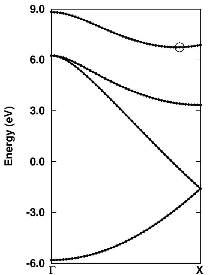
Can you find the Cartesian k-coordinates in units of \tpiba of the valence band maximum (VBM) and conduction band minimum (CBM)? Inspecting file bands.dat, those are:
            0.000000  0.000000  0.000000
-5.811    6.253    6.253    6.253    8.817
...
            0.000000  0.840000  0.000000
-2.783   -0.278    3.440    3.440    6.743
We can see that the VBM lies at the \(\Gamma\)-point and is threefold degenerated with energy \(E_{\rm VBM} = 6.253\) eV. The CBM lies at \(\sim 0.84\) \(\Gamma\)-X with energy \(E_{\rm CBM} = 6.743\) eV. Therefore, the DFT-LDA band gap with these settings is \(E_{\rm G} = E_{\rm CBM} - E_{\rm VBM} = 0.49\) eV.
Step 3
Run a non self-consistent calculation for two K-points that define the VBM and CBM in the equilibrium and ZG supercell structures.
Note: Find the reciprocal lattice vector of the supercell G that maps K onto k, i.e. K \(=\) k \(-\) G. The trivial choice is G \(= \Gamma\) and thus set K \(=\) k.
To prepare the calculation proceed as follows:
cd ../workdir/
cp ../../exercise1/workdir/equil-scf_333.in equil-nscf_333.in
cp ../../exercise1/workdir/ZG-scf_333_0.00K.in ZG-nscf_333_0.00K.in
cp -r ../../exercise1/workdir/equil-si.save/ .
cp -r ../../exercise1/workdir/ZG-0.00K-si.save/ .
In equil-nscf_333.in and ZG-nscf_333_0.00K.in apply the following changes:
Set
calculation = 'nscf'.Include one empty band / unit-cell by setting
nbnd = 135belowecutwfc = 20.0flag.Replace the automatic K-grid:
K_POINTS automatic
2 2 2 0 0 0
with the two K-points of the VBM and CBM:
K_POINTS crystal
2
0.000000 0.000000 0.000000 1
0.000000 1.260000 1.260000 1
Remark: Since the coordinates are given in units of the reciprocal lattice parameters, we obtain the K-coordinates by multiplying the k-coordinates of VBM and CBM with the supercell dimensions, i.e. if k \(= [ x \,\,\, y \,\,\, z]\) then K \(= [ m\times x \,\,\, n\times y \,\,\, p\times z]\), where integers \(m,n,p\) define an \(m\times n \times p\) supercell.
For the ZG input file add
nosym = .true.belownbnd = 135.
optional: If you did not complete exercise1 and the steps above, then copy files from inputs:
cd ../workdir/; cp ../inputs/*nscf_333*in .; cp -r ../inputs/*-si.save/ .
For example, the ZG input file should look like this:
ZG-nscf_333_0.00K.in
 &control
  calculation = 'nscf'
  restart_mode = 'from_scratch'
  prefix = 'ZG-0.00K-si'
  pseudo_dir = './',
  outdir = './'
/
&system
  ibrav = 0, nat =   54, ntyp =    1
  nbnd = 135, ecutwfc =  20.00, nosym = .true.
  occupations = 'fixed',  smearing = 'gaussian',  degauss =   0.0D+00
/
&electrons
  diagonalization = 'david',  mixing_mode= 'plain',
  mixing_beta = 0.70, conv_thr =   0.1D-06
/
ATOMIC_SPECIES
   Si   28.085 Si.pz-vbc.UPF
K_POINTS crystal
2
0.000000 0.000000 0.000000 1
0.000000 1.260000 1.260000 1
CELL_PARAMETERS (angstrom)
     -8.09641133      0.00000000      8.09641133
      0.00000000      8.09641133      8.09641133
     -8.09641133      8.09641133      0.00000000
ATOMIC_POSITIONS (angstrom)
...
mpirun -n 28 $QE/pw.x -nk 2 < equil-nscf_333.in > equil-nscf_333.out
mpirun -n 28 $QE/pw.x -nk 2 < ZG-nscf_333_0.00K.in > ZG-nscf_333_0.00K.out
The calculations should take around 5 secs each. When the equilibrium calculation is finished, check that you obtain the VBM and CBM energies you would expect. To this aim type:
grep highest equil-nscf_333.out
highest occupied, lowest unoccupied level (ev): 6.2534 6.7435
Indeed, we obtain the correct VBM and CBM energies and a gap of 0.4902 eV. To get the band gap from the ZG calculation at 0 K type:
a=$(grep highest ZG-nscf_333_0.00K.out | awk '{print $7}')
grep $a ZG-nscf_333_0.00K.out | head -1  # VBM
5.4332 6.2765 6.2828 6.2912 6.8273 6.8375 6.8609 6.8953
a=$(grep highest ZG-nscf_333_0.00K.out | awk '{print $8}')
grep $a ZG-nscf_333_0.00K.out | head -1  # CBM
5.6192 5.6710 5.8206 5.8362 6.7184 7.2537 7.3388 7.5575
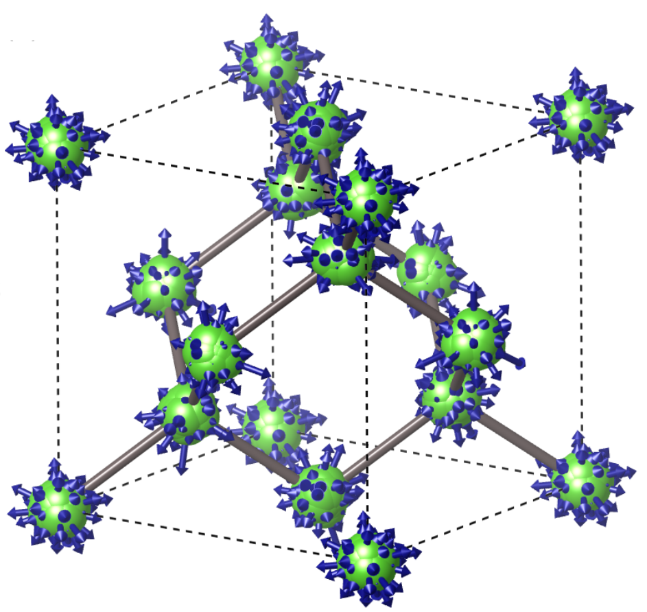
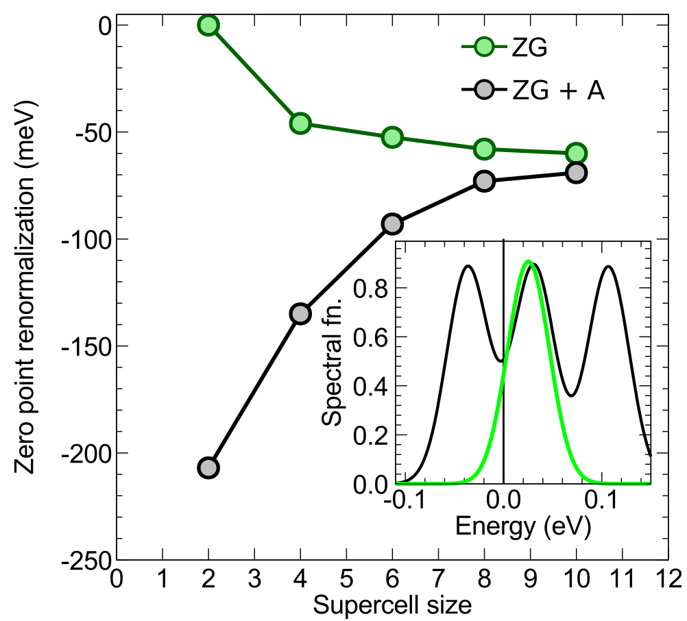
We can see that there is a splitting of the originally threefold degenerated VBM of the order: \(\Delta E = 6.2912 - 6.2835 \simeq 8\) meV. This degeneracy breaking results from the ZG displacements in a finite size supercell and should reduce to zero for larger ZG simulation cells. This is a consequence of the harmonic approximation, where the symmetries of the system should be maintained upon thermal averaging (see thermal ellipsoids in the plot below). We note that for minimizing the effect of band degeneracy splitting we excluded the modes in set \(\mathcal{A}\). In Ref. [Phys. Rev. Res. 2, 013357 (2020)] we show that these modes dominate VBM splitting (see the spectral function in the figure below), giving \(\Delta E > 80\) meV for a \(4\times4\times4\) ZG supercell. Hence, for finite size systems with degenerated band edges, it is suggested to keep incl_qA = .false.. To deal with this finite size supercell artefact, we determine the VBM by taking the average of the three bands as done in the commands above. For example in ZG-nscf_333_0.00K.out, the energy of the VBM is: \(E_{\rm VBM} = (6.2765 + 6.2828 + 6.2912)/3 = 6.2835\) eV. Thus the band gap at 0K is \(E(0 \,{\rm K}) = 6.7184 - 6.2835 = 0.4349\) eV, and we can determine a zero-point renormalization \(E_{\rm ZPR} = 0.4901 - 0.4349 \simeq 55\) meV. This value is in good agreement with literature data (check, for example, Refs. [J. Chem. Phys. 143, 102813 (2015) ] and [New J. Phys. 20, 123008 (2018) ]).
Note: In general, to obtain reliable values of the zero-point renormalization, one should always check convergence with respect to the ZG supercell size (see the right part of the figure below).
Before going to the next step remove unnecessary files:
rm -r *wfc* *save
Step 4
Prepare a band structure unfolding calculation using the \(3\times3\times3\) ZG configuration.
Create a new directory and copy the necessary input files:
mkdir band_structure_unfolding/; cd band_structure_unfolding/
cp ../../inputs/bands_unfold.in bands.in; cp ../../inputs/Si.pz-vbc.UPF .
cp -r ../../../exercise1/workdir/ZG-0.00K-si.save/ .
cp ../ZG-nscf_333_0.00K.in ZG-bands_333_0.00K.in
In ZG-bands_333_0.00K.in apply the following modifications:
Set
calculation = 'bands'Replace the following lines containing information about the K-points:
K_POINTS crystal
2
0.000000 0.000000 0.000000 1
0.000000 1.260000 1.260000 1
with
K_POINTS crystal_b
2
0.000000 0.000000 0.000000 35
0.000000 1.500000 1.500000 1
Note: Here we choose to sample the \(\Gamma\)-X path with 36 equally-spaced K-points.
If you did not complete the previous step, then copy:
cp ../../inputs/ZG-bands_333_0.00K.in .
The file ZG-bands_333_0.00K.in should look like this:
ZG-bands_333_0.00K.in
&control
  calculation = 'bands'
  restart_mode = 'from_scratch'
  prefix = 'ZG-0.00K-si'
  pseudo_dir = './'
  outdir = './'
/
&system
  ibrav = 0
  nat =   54
  ntyp =    1
  nbnd = 135, nosym = .true., ecutwfc =  20.00
  occupations = 'fixed'
  smearing = 'gaussian'
  degauss = 0.0D+00
/
&electrons
  diagonalization = 'david'
  mixing_mode= 'plain'
  mixing_beta = 0.70
  conv_thr =   0.1D-06
/
ATOMIC_SPECIES
   Si   28.085 Si.pz-vbc.UPF
K_POINTS crystal_b
2
0.000000 0.000000 0.000000 35
0.000000 1.500000 1.500000 1
CELL_PARAMETERS {angstrom}
     -8.09641133      0.00000000      8.09641133
      0.00000000      8.09641133      8.09641133
     -8.09641133      8.09641133      0.00000000
ATOMIC_POSITIONS {angstrom}
...
We also show here the file bands.in:
bands.in
&bands
 prefix  = 'ZG-0.00K-si'
 outdir  = './'
 filband = 'bands.dat'
 lsym    = .false.
 dim1    = 3,
 dim2    = 3,
 dim3    = 3
/
Note: The input variables in bands.in are the same as in a standard bands.x calculation. The only difference is the flags dimX used to specify the dimensions of the ZG supercell.
Step 5
Run a band structure unfolding calculation.
mpirun -n 48 $QE/pw.x -nk 12 < ZG-bands_333_0.00K.in > ZG-bands_333_0.00K.out
mpirun -n 28 $QE/bands_unfold.x < bands.in > bands.out
The bands calculation should take around 40 secs and the unfolding around 4 secs. Now read the outputs of bands01.dat and spectral_weights01.dat. Can you guess what’s the meaning of the spectral weights for each band?
head -16 bands01.dat
&plot nbnd= 135, nks=    36 /
           0.000000  0.000000  0.000000
    -5.835502     -4.538594     -4.530763     -4.523530     -4.499082   ...
    -3.908153     -3.894924     -3.872739     -3.810481     -3.778147   ...
    -2.482541     -2.472723     -2.444686     -2.416635     -2.374668   ...
    -0.601738     -0.585920     -0.573318     -0.535188     -0.508788   ...
     0.770211      0.785536      0.830510      0.877961      0.890418   ...
     1.270759      1.327158      1.332847      1.629158      1.634093   ...
     ...
head -16 spectral_weights01.dat
&plot nbnd= 135, nks=    36 /
           0.000000  0.000000  0.000000
   0.988833    0.000257    0.000674    0.004029    0.000067    ...
   0.000272    0.000063    0.000675    0.000295    0.000317    ...
   0.000381    0.000283    0.000135    0.000132    0.000134    ...
   0.000072    0.000161    0.000127    0.000191    0.000317    ...
   0.000172    0.000207    0.000168    0.000157    0.000201    ...
   0.000211    0.000183    0.000078    0.000132    0.000125    ...
   ...
Can you spot the weights corresponding to the VBM? What would the weights be if we use the equilibrium \(3\times3\times3\) supercell? In this case, one should obtain the perfect unfolding reproducing the unit cell band structure. The data in the files bands01.dat and spectral_weights01.dat, represent the band energies, \(\varepsilon_{m {\bf K}}(T)\), and spectral weights, \(P_{m {\bf K}, {\bf k}} (T)\), for all K-points, respectively.
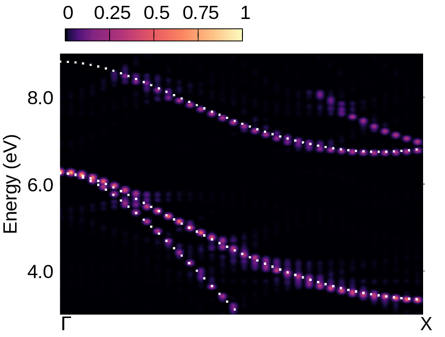
Now you have all the ingredients to evaluate the spectral function \(A_{\bf k}(\varepsilon,T) = \sum_{m {\bf K}} P_{m {\bf K}, {\bf k}} (T) \delta [\varepsilon - \varepsilon_{m {\bf K}}(T)]\).
Step 6
Calculate the spectral function using the energies and spectral weights. To this aim convert first bands01.dat and spectral_weights01.dat into a different format using plotband.x of QE:
cp ../../inputs/energies.in .
cp ../../inputs/spectral_weights.in .
$QE/plotband.x spectral_weights01.dat < spectral_weights.in > spw.out
$QE/plotband.x bands01.dat < energies.in > energies.out
sed -i '/^\s*$/d' spectral_weights.dat # remove empty lines
sed -i '/^\s*$/d' energies.dat # remove empty lines
paste energies.dat spectral_weights.dat > tmp
awk '{print $1,$2,$4}' tmp > energies_weights.dat; rm tmp
You have just generated energies_weights.dat file in a similar format to a “.gnu” file where the first column has the momentum-axis values, the second the energies, and the third the spectral weights. Now proceed with the calculation of the spectral function using pp_spctrlfn.x:
cp ../../inputs/energies_weights.dat . # If you missed the step above
cp ../../inputs/pp_spctrlfn.in .
mpirun -n 4 $QE/pp_spctrlfn.x -nk 4 < pp_spctrlfn.in > pp_spctrlfn.out
The file pp_spctrlfn.in takes the following input variables:
pp_spctrlfn.in
&input
  flin = 'energies_weights.dat'
  steps = 4860,
  ksteps = 200,
  esteps = 200,
  kmin = 0,
  kmax = 0.7071,
  emin =  3.00
  emax = 9.00
  flspfn = 'spectral_function.dat'
/
Here, (i) steps is the number of rows in the input file flin, (ii) ksteps and esteps define the resolution of the spectral function along the momentum-axis and energy-axis, (iii) (kmin-kmax) and (emin-emax) define the momentum and energy windows, and (iv) in flspfn we provide the name of the output file.
Now plot the spectral function:
cp spectral_function.dat ../../gnuplot/. ; cd ../../gnuplot/
cp ../inputs/bands.dat.gnu .
gnuplot gp_pm3d.p; evince bsu_si_0K.pdf
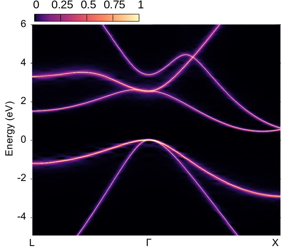
We also copied bands.dat.gnu for comparing the spectral function with the band structure calculated with the atoms at their equilibrium positions (white lines in the plots below) - note also that we assign a spectral weight of 1.0 in the third column of bands.dat.gnu. In the right part of the figure below, we also reproduced the converged calculation from Ref. [Phys. Rev. Res. 2, 013357 (2020)], employing an \(8\times8\times8\) ZG supercell, more K-points and empty bands.
In APPENDIX / Exercise 2 we provide a recipe for performing band structure unfolding for each K-point separately. This approach is most effective when larger supercells are employed and pw.x cannot handle all K-points in one run.
Exercise 3
In this exercise we will learn how to calculate the phonon-assisted optical spectra using the example of silicon and the \(3\times3\times3\) ZG supercell for \(T=0\) K. To obtain temperature-dependent optical spectra we will evaluate the optical matrix elements in the independent-particle approximation using a routine very similar to epsilon.x of QE. We emphasize that this methodology can be extended to higher-level theories of optical absorption, like RPA, BSE, etc … The present approach of calculating phonon-assisted optical spectra is based on Ref. [Phys. Rev. B 94, 075125 (2016)].
Note: The calculation of phonon-assisted optical spectra using ZG configurations has some drawbacks and advantages when compared to the perturbative methodologies, e.g. QDPT, implemented in EPW. First go to the directory exercise3, create your working directories and copy the input files:
cd ../../exercise3/; mkdir workdir; cd workdir; mkdir equil; mkdir ZG
cd equil
cp ../../inputs/equil/K_list.in .
cp ../../inputs/equil/epsilon.in .
cp -r ../../../exercise1/workdir/equil-si.save/ .
cp ../../../exercise2/workdir/equil-nscf_333.in .
The file K_list.in contains the crystal coordinates of 200 randomly generated K-points. We use random K-points, instead of a uniform grid, in order to speed up convergence. In equil-nscf_333.in apply the following changes:
1. Add nosym = .true. below nbnd = 135.
Note: although we use the equilibrium structure we set nosym = .true. since random K-points are employed.
Delete the information for the K-points:
K_POINTS crystal 2
0.000000 0.000000 0.000000 1
0.000000 1.260000 1.260000 1
and at the bottom of the file add the following:
K_POINTS crystal 30
Copy and paste the first 30 K-points from file
K_list.in.
If you did not complete Exercise 1 and Exercise 2, you can copy:
cp ../../inputs/equil/equil-nscf_333.in .
cp -r ../../../exercise2/inputs/equil-si.save/ .
The file equil-nscf_333.in should look like this:
equil-nscf_333.in
&control
  calculation = 'nscf'
  restart_mode = 'from_scratch'
  prefix = 'equil-si'
  pseudo_dir = './'
  outdir = './'
/
&system
  ibrav = 0
  nat =   54
  ntyp =    1
  ecutwfc =  20.00
  nbnd = 135
  nosym = .true.
  occupations = 'fixed'
  smearing = 'gaussian'
  degauss =   0.0D+00
/
&electrons
  diagonalization = 'david'
  mixing_mode= 'plain'
  mixing_beta = 0.70
  conv_thr =   0.1D-06
/
ATOMIC_SPECIES
   Si   28.085 Si.pz-vbc.UPF
CELL_PARAMETERS {angstrom}
     -8.09641133      0.00000000      8.09641133
      0.00000000      8.09641133      8.09641133
     -8.09641133      8.09641133      0.00000000
ATOMIC_POSITIONS {angstrom}
   Si    0.00000000   0.00000000   0.00000000
   Si   -2.69880378   0.00000000   2.69880378
...
K_POINTS crystal
30
0.236650 0.022946 0.917156 1.0
0.392728 0.655175 0.471114 1.0
...
We also show here the file epsilon.in:
epsilon.in
&inputpp
outdir      = './',
prefix      = 'equil-si',
calculation = 'eps'
/
&energy_grid
smeartype   = 'gauss',
intersmear  = 0.03d0,
wmax        = 4.5d0,
wmin        = 0.2d0,
nw          = 600,
shift       = 0.0d0,
/
Note: The input variables in epsilon.in are the same as in a standard epsilon.x calculation.
Step 1
Run an optical spectrum calculation for silicon using the \(3\times3\times3\) equilibrium supercell and 30 random K-points. The aim is to calculate the imaginary part of the dielectric function, see e.g. Ref. [Phys. Rev. B 94, 075125 (2016)]. To calculate the dielectric function we use epsilon_Gaus.x, which is a slightly modified routine of epsilon.x, that replaces the delta function with a Gaussian instead of a Lorentzian function. We choose to apply Gaussian broadening in order to minimize numerical artefacts at the absorption onset.
mpirun -n 48 $QE/pw.x -nk 24 < equil-nscf_333.in > equil-nscf_333.out
mpirun -n 24 $QE/epsilon_Gaus.x < epsilon.in > epsilon.out
rm *wfc* *save/*wfc*
The full calculation should take around 50 secs. The output files are (i) epsi_equil-si.dat containing \(\epsilon_2(\omega)\), (ii) epsr_equil-si.dat containing the real part of the dielectric function \(\epsilon_1(\omega)\), and (iii) eels_equil-si.dat containing the electron energy loss spectrum; all calculated for the equilibrium structure. In each file the first column is the energy grid, and the rest three represent the observable along the three Cartesian directions.
Step 2
Take the isotropic average of the dielectric function and copy the output file in the gnuplot directory using:
awk '{print $1,($2+$3+$4)/3}' epsi_equil-si.dat > epsi_si_333_equil_30_av.dat
cp epsi_si_333_equil_30_av.dat ../../gnuplot/.
Step 3
Run an optical spectra calculation for silicon using the \(3\times3\times3\) ZG supercell and 30 random K-points. We will essentially repeat all steps performed for calculating the optical spectra of the \(3\times3\times3\) equilibrium supercell. First go to the ZG directory and copy the input files:
cd ../ZG/
cp ../../inputs/ZG/K_list.in .
cp ../../inputs/ZG/epsilon.in .
cp -r ../../../exercise1/workdir/ZG-0.00K-si.save/ .
cp ../../../exercise2/workdir/ZG-nscf_333_0.00K.in .
In ZG-nscf_333_0.00K.in apply the following change:
Delete the information for the K-points:
K_POINTS crystal
2
0.000000 0.000000 0.000000 1
0.000000 1.260000 1.260000 1
and at the bottom of the file add the following:
K_POINTS crystal
30
Copy and paste the first 30 K-points from file
K_list.in.
If you did not complete Exercise 1 and Exercise 2, copy ZG-0.00K-si.save and ZG-nscf_333_0.00K.in from:
cp ../../inputs/ZG/ZG-nscf_333_0.00K.in .
cp -r ../../../exercise2/inputs/ZG-0.00K-si.save/ .
The file ZG-nscf_333_0.00K.in should look like this:
ZG-nscf_333_0.00K.in
&control
  calculation = 'nscf'
  restart_mode = 'from_scratch'
  prefix = 'ZG-0.00K-si'
  pseudo_dir = './'
  outdir = './'
/
&system
  ibrav = 0
  nat =   54
  ntyp =    1
  ecutwfc =  20.00
  nbnd = 135
  nosym = .true.
  occupations = 'fixed'
  smearing = 'gaussian'
  degauss =   0.0D+00
/
&electrons
  diagonalization = 'david'
  mixing_mode= 'plain'
  mixing_beta = 0.70
  conv_thr =   0.1D-06
/
ATOMIC_SPECIES
   Si   28.085 Si.pz-vbc.UPF
CELL_PARAMETERS {angstrom}
     -8.09641133      0.00000000      8.09641133
      0.00000000      8.09641133      8.09641133
     -8.09641133      8.09641133      0.00000000
ATOMIC_POSITIONS {angstrom}
...
K_POINTS crystal
30
  0.236650 0.022946 0.917156 1.0
  0.392728 0.655175 0.471114 1.0
...
epsilon.in is the same with the one used before, but with prefix = 'ZG-0.00K-si'.
Step 4
Now run the following to calculate \(\epsilon_2(\omega)\) at 0.00 K:
mpirun -n 48 $QE/pw.x -nk 24 < ZG-nscf_333_0.00K.in > ZG-nscf_333_0.00K.out
mpirun -n 24 $QE/epsilon_Gaus.x < epsilon.in > epsilon.out
The full calculation should take around 50 secs. The output files are (i) epsi_ZG-0.00K-si.dat containing \(\epsilon_2(\omega)\), (ii) epsr_ZG-0.00K-si.dat containing the real part of the dielectric function \(\epsilon_1(\omega)\), and (iii) containing the electron energy loss spectrum eels_ZG-0.00K-si.dat; all calculated for \(T = 0.00\) K. In each file the first column is the energy grid, and the rest three represent the temperature-dependent observable along the three Cartesian directions.
Step 5
Take the isotropic average of the dielectric function and copy the output file in the gnuplot directory using:
awk '{print $1,($2+$3+$4)/3}' epsi_ZG-0.00K-si.dat > epsi_si_333_ZG_30_av.dat
cp epsi_si_333_ZG_30_av.dat ../../gnuplot/.
rm *wfc* *save/*wfc*
The output file containing the data is epsi_si_333_ZG_30.dat.
Now go to the gnuplot directory and plot ZG and equilibrium spectra using:
cd ../../gnuplot/; gnuplot gp_coms.p; evince ZG_spectra.pdf
gnuplot gp_coms_logscale.p; evince ZG_spectra_logscale.pdf
We also plot \(\varepsilon_2(\omega)\) as calculated with more K-points to obtain convergence.
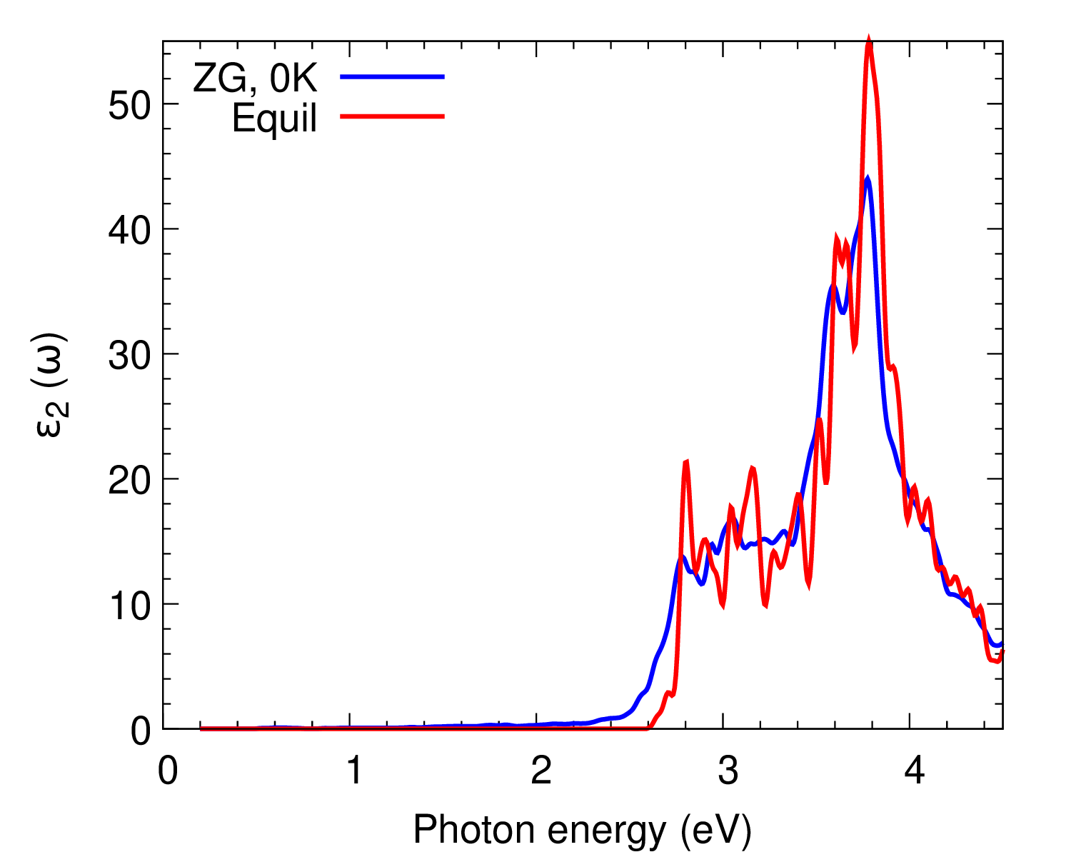
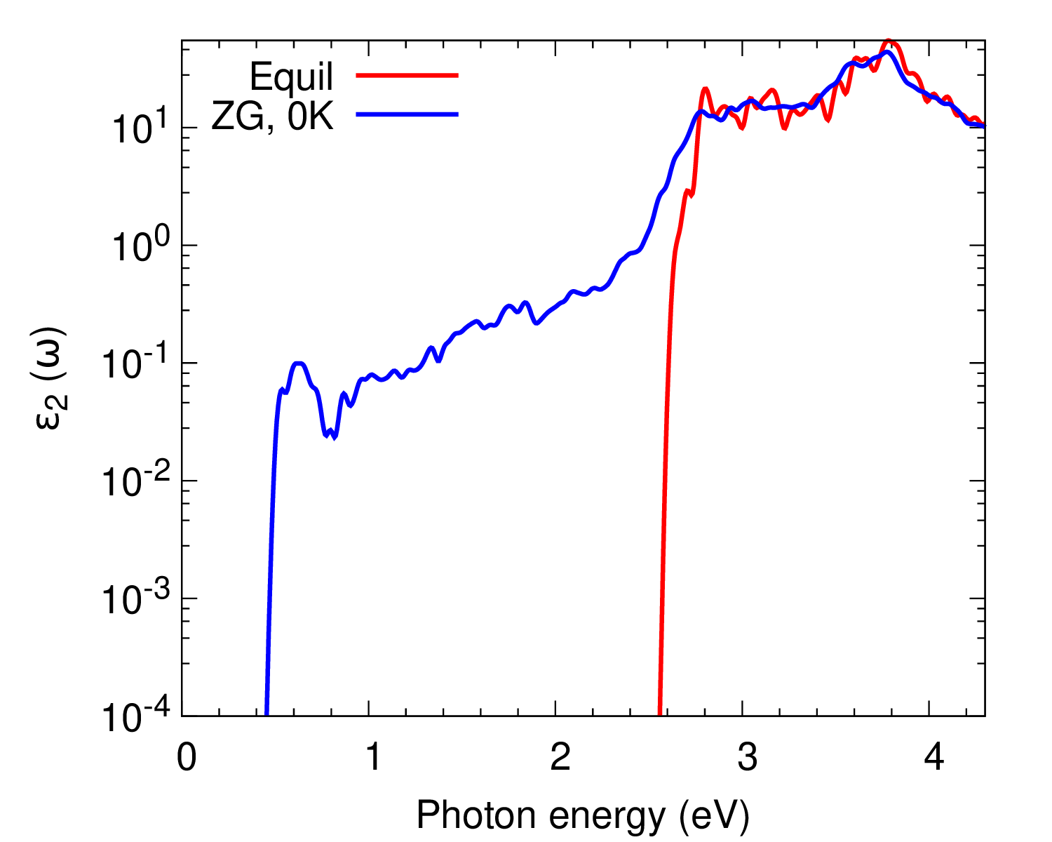
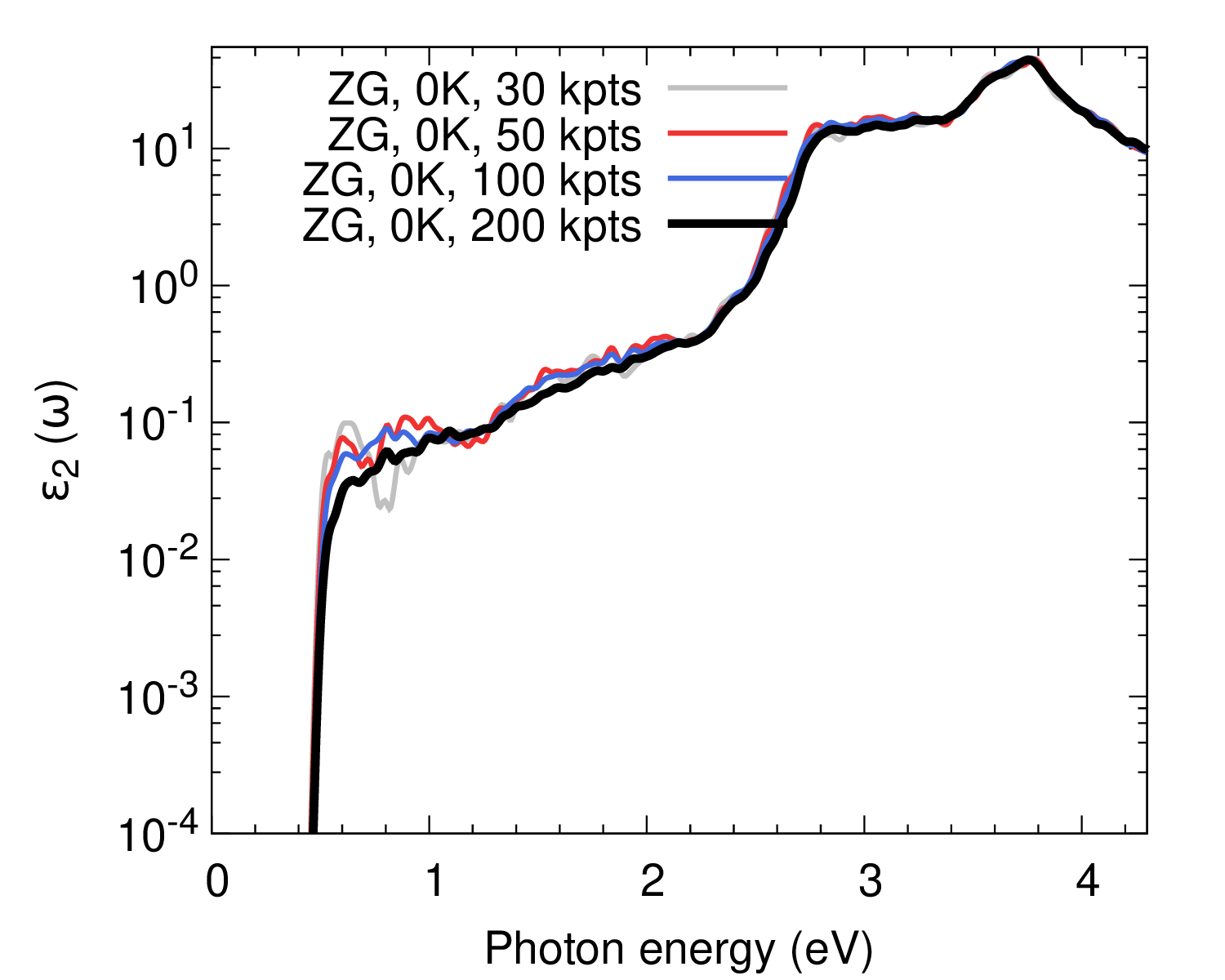
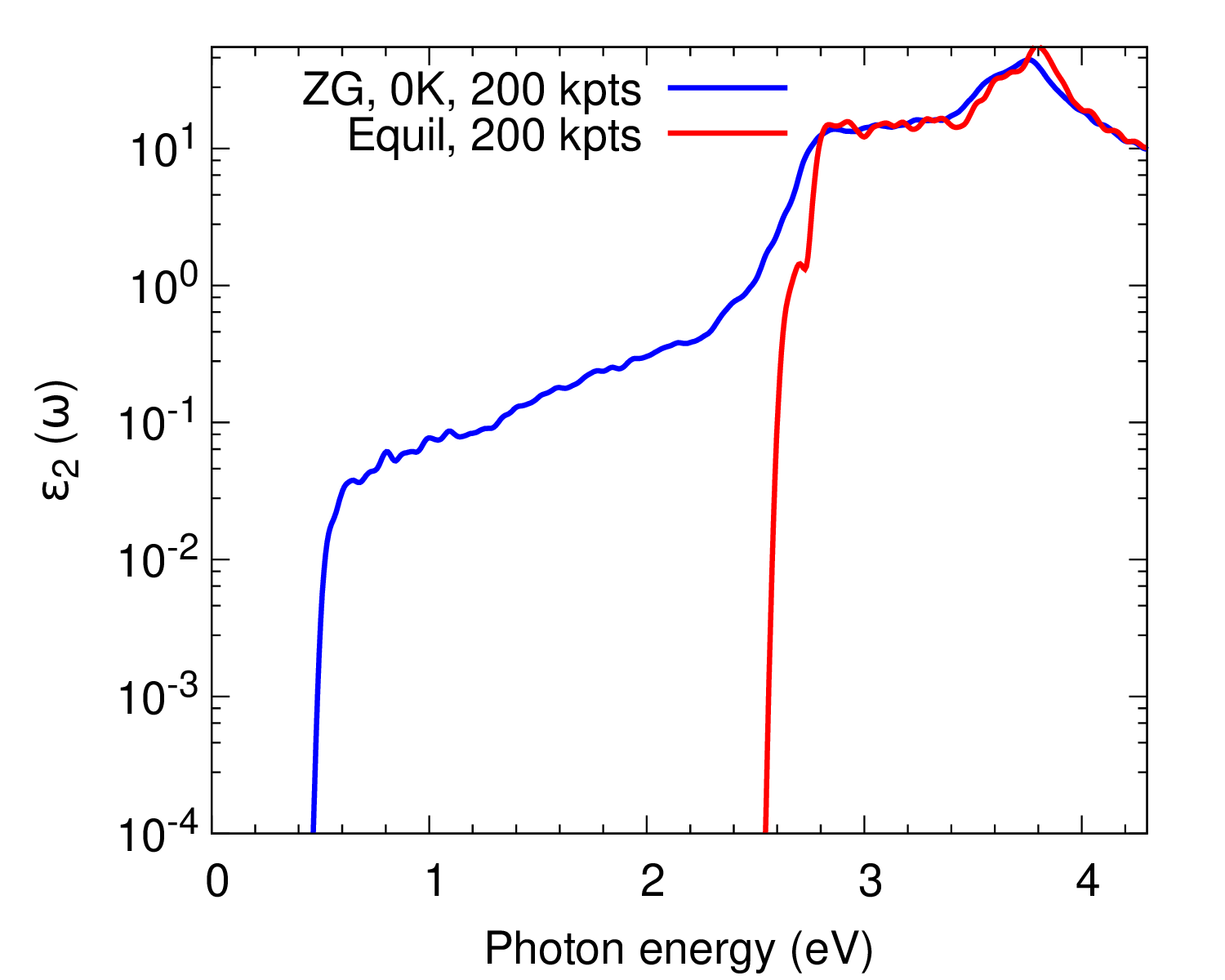
What are the differences between the ZG and equilibrium spectra? Are phonon-assisted transitions captured as expected?
As a homework, repeat the calculation with more random K-points using those provided in the file K_list.in. The result should look like as in the bottom panel of the figure above.
Ref. [Phys. Rev. B 94, 075125 (2016)] reports the convergence of the spectra with respect to the ZG supercell size and the agreement with experimental data for the absorption coefficient.
In APPENDIX / Exercise 3 we provide a recipe for calculating optical spectra for each K-point separately. This approach is most effective when larger supercells are employed and pw.x cannot handle all K-points at once.
Exercise 4
In this exercise we will learn how to calculate temperature-dependent gap renormalizations in the harmonic approximation with SDM, using the example of the direct gap of diamond. We will employ \(4\times4\times4\) ZG supercells. We will also show how to calculate the free energy of the system as a function of temperature. To handle multiple temperatures, we introduce the flag T_array(X) in the ZG code. For consistency reasons, the code assigns the first choice of signs generated without minimizing the error function \(E(\{S_{{\bf q} \nu}\})\), i.e. sets compute_error = .false.. A prerequisite for understanding the workflow in this exercise is to complete Exercise 1 for silicon.
Step 1
Go to the directory exercise4, create workdir, copy script.sh from inputs, and submit:
cd exercise4/; mkdir workdir; cd workdir
cp ../inputs/script.sh .
sbatch script.sh
The script will (i) run scf and DFPT phonon calculations to obtain the harmonic phonons of diamond within the unit cell, (ii) generate ZG configurations for multiple temperatures with ZG.x, (iii) run scf calculations for the equilibrium and ZG structures, (iv) prepare and run nscf calculations for the equilibrium and ZG structures, and (v) extract the temperature dependent direct gap. The commands and workflow in the submission script script.sh are provided in this link. The script should take around 18 minutes to finish, so while it’s running proceed to the following. Remember to modify the script based on your HPC environment.
The files scf.in, ph.in, q2r.in, and matdyn.in are provided here:
scf.in
 &control
    calculation = 'scf'
    restart_mode = 'from_scratch',
    prefix = 'scf',
    pseudo_dir = './',
    outdir='./'
 /
 &system
    ibrav = 2,
    celldm(1) = 6.75,
    nat =  2,
    ntyp = 1,
    ecutwfc = 50.0
 /
 &electrons
    diagonalization='david'
    mixing_mode = 'plain'
    mixing_beta = 0.7
    conv_thr = 1.0d-7
 /
ATOMIC_SPECIES
 C  12.011  C.upf
K_POINTS automatic
6 6 6 0 0 0
ATOMIC_POSITIONS {crystal}
 C 0.00 0.00 0.00
 C 0.25 0.25 0.25
ph.in
&inputph
   amass(1)= 12.011,
   prefix = 'scf'
   outdir = './'
   fildyn = 'C.dyn'
   tr2_ph = 1.0d-12, ldisp = .true.
   nq1 = 2,   nq2 = 2,   nq3 = 2
/
q2r.in
&input
 fildyn='C.dyn', flfrc = 'C.fc'
/
matdyn.in
&input
    asr='all', amass(1)= 12.011,
    flfrc='C.fc', fldyn='C.dyn.mat', flfrq='C.freq', fleig='C.dyn.eig',
    q_in_cryst_coord = .false., q_in_band_form = .true.
/
 9
 0       0       0      100
 0.75    0.75    0.0    1
 0.25    1.00    0.25   100
 0.00    1       0.00   100
 0       0       0      100
 0.50    0.50    0.50   100
 0       1       0      100
 0.50    1.00    0      100
 0.50    0.50    0.50   100
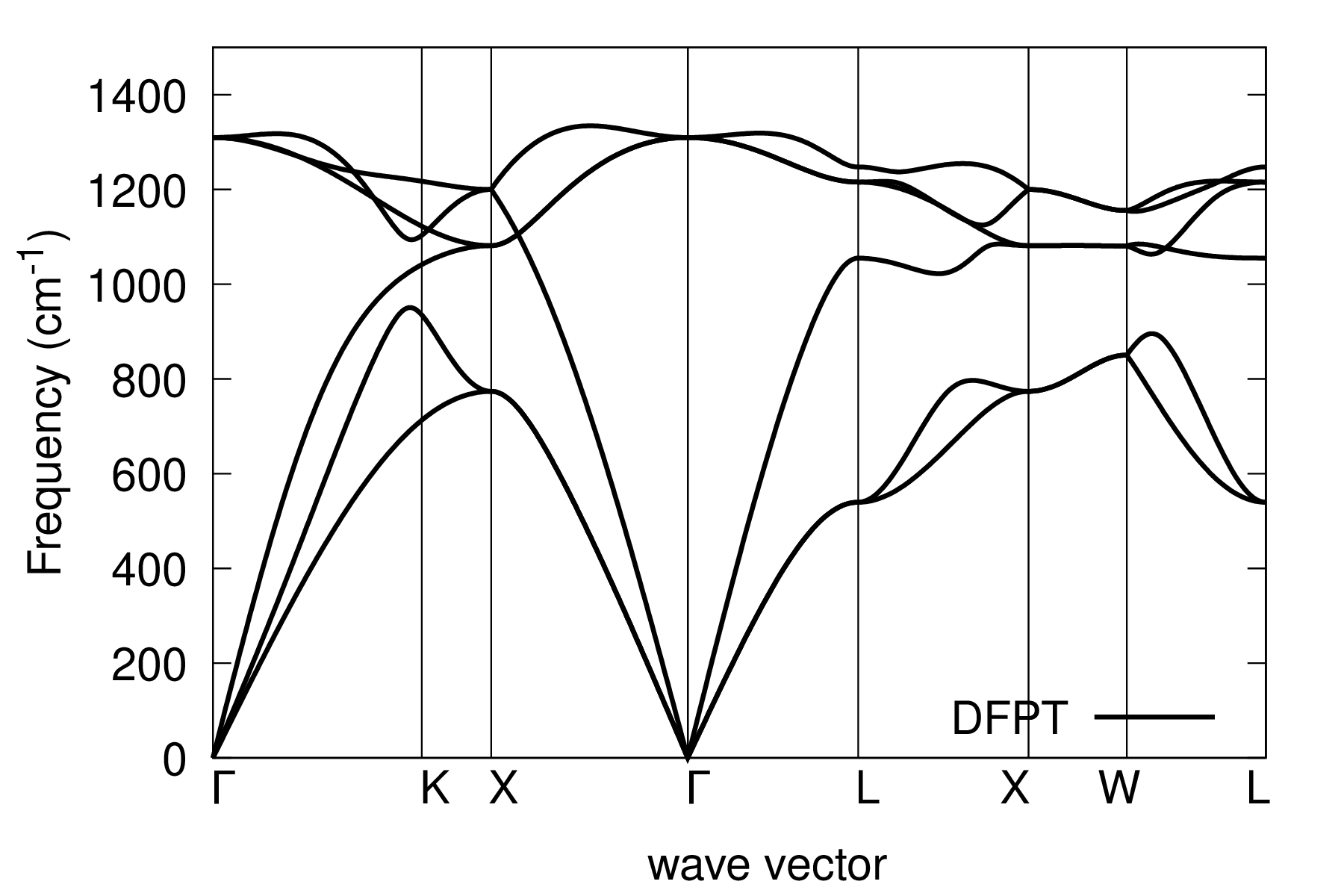
We also note that the calculations are performed with unconverged settings (e.g. cutoff, k-point and q-point grids). Results for converged settings are provided in Ref. [Phys. Rev. B 94, 075125 (2016)].
The ZG file used (ZG_444_multi_T.in) looks like:
ZG_444_multi_T.in
&input
    flfrc='C.fc', flscf = 'scf.in'
    asr='all', amass(1)=12.011, atm_zg(1) = 'C',
    T_array(1) = 0, T_array(2) = 50, T_array(3) = 100, T_array(4) = 150
    T_array(5) = 200, T_array(6) = 250, T_array(7) = 300,  T_array(8) = 350,
    T_array(9) = 400, T_array(10) = 600, T_array(11) = 800, T_array(12) = 1000
    dim1 = 4, dim2= 4, dim3 = 4, incl_qA = .false.
    compute_error = .true., synch =.true., error_thresh = 0.1, niters = 100
/
Note: C.fc contains the harmonic IFCs. T_array(X) allows ZG configurations for multiple temperatures.
Step 2
Use plotband.x to obtain the data for the phonon dispersion:
$QE/plotband.x
Input file > C.freq
Reading    6 bands at    702 k-points
Range:    0.0000 1334.1534eV  Emin, Emax, [firstk, lastk] > 0 1400
high-symmetry point:  0.0000 0.0000 0.0000   x coordinate   0.0000
high-symmetry point:  0.7500 0.7500 0.0000   x coordinate   1.0607
high-symmetry point:  0.2500 1.0000 0.2500   x coordinate   1.0607
high-symmetry point:  0.0000 1.0000 0.0000   x coordinate   1.4142
high-symmetry point:  0.0000 0.0000 0.0000   x coordinate   2.4142
high-symmetry point:  0.5000 0.5000 0.5000   x coordinate   3.2802
high-symmetry point:  0.0000 1.0000 0.0000   x coordinate   4.1463
high-symmetry point:  0.5000 1.0000 0.0000   x coordinate   4.6463
high-symmetry point:  0.5000 0.5000 0.5000   x coordinate   5.3534
output file (gnuplot/xmgr) > C_harm_ph_dispersion.xmgr
bands in gnuplot/xmgr format written to file C_harm_ph_dispersion.xmgr
output file (ps) >
stopping ...
Step 3
Now plot the phonon dispersion using:
gnuplot gp_coms.p
evince C_ph_dispersion.pdf
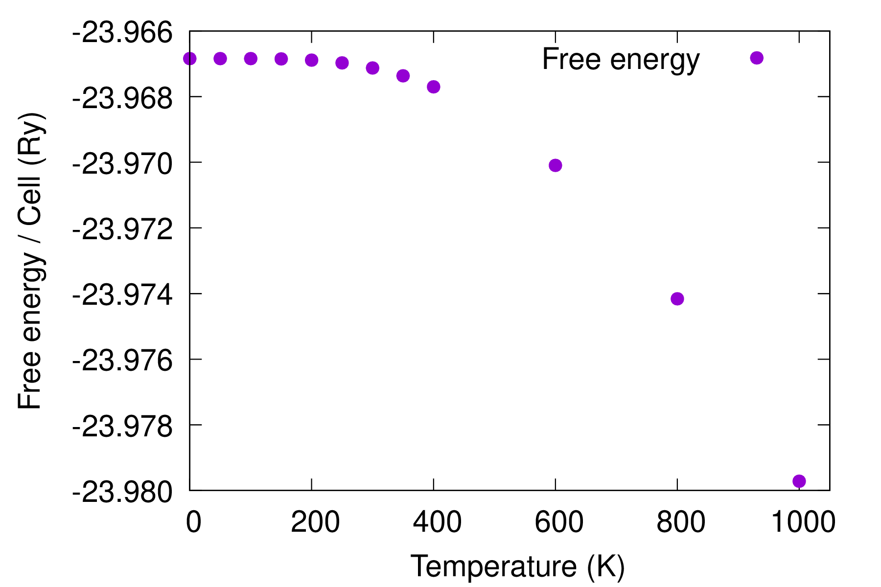
Step 4
Plot the free energy of diamond ZG configurations given by \(F = \braket{U}_T - T S\), where \(U\) is the total energy of the system and \(S\) is the entropy. The last line is essentially equivalent to Eq. (10) of Ref. [Phys. Rev. B 108, 035155 (2023)]; for definitions please check therein. This equation contains the total energy of the system at thermal equilibrium evaluated with the nuclei clamped at their ZG coordinates, the potential vibrational energy and the vibrational free energy. The total energy of the system at thermal equilibrium is obtained after a DFT calculation using the ZG configuration. The potential vibrational energy and the vibrational free energy are printed by the code in ZG_444_multi_T.out.
Step 5
Run the commands below one by one and spot each term in the outputs:
grep "Potential" ZG_444_multi_T.out | awk '{print $3}' > Pot_ene.dat
grep "free ene" ZG_444_multi_T.out | awk '{print $4}' > Vib_free_ene.dat
grep ! ZG-scf_444_* | awk '{print $1,$5}' > tmp
sed 's/ZG-scf_444_//g' tmp | sed 's/K.out:!//g' > tmp2 # remove strings
sort -k1n tmp2 > Tot_ene.dat
paste Tot_ene.dat Pot_ene.dat Vib_free_ene.dat > data.dat
gnuplot gp_coms_free.p; evince C_free_energy.pdf
Step 6
If the calculation is completed, plot the direct gap renormalization of diamond and compare with experiment.
gnuplot gp_coms_gap.p; evince C_Renormalization_T.pdf
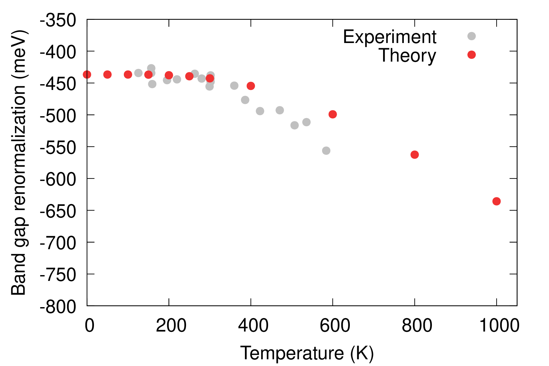
The DFT direct gap of diamond at static-equilibrium is
cat eq_direct_gap.dat
5.5464 # eV
The DFT-ZG direct gap of diamond at finite temperatures is:
cat direct_gap_T_av.dat
# T (K)  Dir. gap (eV)
   0     5.1097
   50    5.1097
   100   5.1097
   150   5.1095
   200   5.1086
   250   5.107
   300   5.1037
   400   5.0918
   600   5.0472
   800   4.9838
   1000  4.9106
Here our calculations yield a zero-point renormalization of \(\Delta E^{\rm dir}_{\rm g} (0\,{\rm K}) = 5.5464 - 5.1097 = 437\) meV for the direct gap of diamond, in good agreement with literature data reported in Table 1 of Ref. [Phys. Rev. B 94, 075125 (2016)]. To obtain the direct gap we (i) identify that the first direct gap of diamond lies at the \(\Gamma\) point of the unit cell’s Brillouin zone, this can be seen by inspecting the file bands.out; both the VBM and CBM defining the direct gap are triply degenerate with values 13.3502 and 18.8956 eV, respectively, (ii) identify the same states calculated for the supercell with atoms at static-equilibrium in file equil-nscf_444.out, (iii) identify the corresponding states calculated for the supercell with atoms at ZG coordinates in files ZG-nscf_444_T.00K.out, and (iv) take the average of the corresponding three valence states and the three conduction states in files ZG-nscf_444_T.00K.out (see script com_av_gap.sh provided in this link). Note that states near the CBM defining the indirect gap of diamond (lying at \(\sim\) 0.8 \(\Gamma\)-X of the unit cell’s Brillouin zone) are folded at the \(\Gamma\)-point of the \(4\times4\times4\) supercell and should be excluded from the analysis (e.g. value 17.6921 eV in equil-nscf_444.out). Our calculations for the temperature-dependent direct gap of diamond compare well with experimental data from Ref. [Phys. Rev. B 46, 4483 (1992)]; note that experimental data are shifted in gp_coms_gap.p to ease comparison with theory.
Exercise 5
In this exercise we will discuss the physical meaning of the ZG configuration and learn how to calculate phonon-induced diffuse (or inelastic) scattering patterns using graphene. This is an example of an observable which allows us to computationally reach the thermodynamic limit and assess multi-phonon processes. More details about the theory of phonon-induced inelastic scattering and its connection to the special displacement method can be found in Ref. [Phys. Rev. B 104, 205109 (2021)].
We will evaluate the exact expression for the all-phonon inelastic scattering intensity and compare it with the ZG scattering intensity, i.e. when the scatterers (nuclei) are defined by the ZG displacements. Go to the directory exercise5, create your working directories, and copy the input files:
cd exercise5; mkdir workdir; cd workdir; mkdir exact; mkdir ZG
cd exact
cp ../../inputs/exact/graphene.881.fc .
cp ../../inputs/exact/disca.in .
Note: The file graphene.881.fc contains the IFC of graphene calculated using an \(8\times8\times1\) q-grid.
Step 1
Run a diffuse scattering calculation using disca.x and the input:
disca.in
&input
    asr = 'all', amass(1) = 12.011, flfrc = 'graphene.881.fc', atm_zg(1) = 'C',
    dim1 = 40, dim2 = 40, dim3 = 1,
    T = 300,
    atmsf_a(1,1) = 0.1361,
    atmsf_a(1,2) = 0.5482,
    atmsf_a(1,3) = 1.2266,
    atmsf_a(1,4) = 0.5971,
    atmsf_a(1,5) = 0.0,
    atmsf_b(1,1) = 0.3731,
    atmsf_b(1,2) = 3.2814,
    atmsf_b(1,3) = 13.0456,
    atmsf_b(1,4) = 41.0202,
    atmsf_b(1,5) = 0.0,
    zero_one_phonon = .true., full_phonon = .true.
    nks1 = 0,  nks2 = 0,  nks3 = 0, nksf1 = 5, nksf2 = 5, nksf3 = 1,
    plane_val = 0.d0, plane_dir = 3
    qstart = 1, qfinal = 40000,
/
&pp_disca
    nrots = 6,
    kres1 = 250,
    kres2 = 250,
    kmin  = -10,
    kmax  = 10,
    col1  = 1,
    col2  = 2,
    Np    = 1600
/
mpirun -np 48 $QE/disca.x -nk 48 < disca.in > disca.out
The input format of disca.in is similar to ZG_333.in. Line 3 contains input variables similar to those in matdyn.in; in line 3 we provide the dimensions dimX of the \({\bf q}\)-grid used to sample the Brillouin zone; in line 4 we provide the temperature T in Kelvin; lines 5-14 contain the parameters of the atomic scattering factor (atmsf(i,j):atmsf_a and atmsf_b) from Ref. [Micron 30, 625–648, (1999)]; in line 15 we specify whether we want to compute the one-phonon (zero_one_phonon) and/or all-phonon (full_phonon) structure factor; in line 16 nks1, nks2, nks3 and nksf1, nksf2, nksf3 define the range of reciprocal lattice vectors (in crystal coordinates) which are used to determine the extent of the calculated scattering vectors (Q-points); in line 17 we provide plane_val that defines the plane along which the structure factor is calculated (in units of 2pi/alat) and plane_dir defines the Cartesian direction perpendicular to the plane (where 1 --> x, 2 --> y, and 3 --> z); and in line 18 we specify the range of Q-points (from qstart to qfinal) for which the structure factor is calculated.
In the namelist &pp_disca we have: (i) nrots which is the number of rotations to be applied on the all-phonon scattering intensity to obtain the complete map. nrots is based on the space group of each system. This step is important to avoid the extra effort of calculating the scattering intensity for wavevectors connected by rotation symmetry (see also plots at the end of the exercise). (ii) kresX:kres1 and kres2 define the resolution of the scattering intensity along the chosen Cartesian axes, (iii) colX:col1 and col2 are integers defining two of the Cartesian directions of the scattering vectors (where 1 --> x, 2 --> y, and 3 --> z), (iv) (kmin - kmax) define the 2D momentum window in reciprocal space, and (v) Np is the number of reduced wavevectors (q-points) used to sample each Brillouin zone.
The standard outputs from a disca.x run are: strf_one-ph_broad.dat and strf_all-ph_broad.dat containing the zero+one-phonon, and all-phonon scattering intensities, respectively, after convolution is applied. These files have three columns: the first two represent the Cartesian coordinates of the scattering vectors and the third column is the scattering intensity.
One can also print for each case the mode resolved and atom resolved scattering intensities by setting mode_resolved = .true. and/or atom_resolved = .true..
For printing the raw data, i.e. before convolution is applied, one can use print_raw_data = .true. to obtain the following data: Bragg_scattering.dat, strf_one-phonon.dat, strf_q_nu_one-phonon.dat, and strf_all-phonon.dat, containing the Bragg, mode (or branch) resolved, one-phonon, and all-phonon scattering intensities, respectively. These files have four columns: the first three represent the Cartesian coordinates of the scattering vectors (\(Q_x\), \(Q_y\), and \(Q_z\)) and the fourth column is the scattering intensity. The code pp_disca.x in EPW/ZG/src can be used separately to convolute the raw data. disca.x also prints the Q vectors in crystal coordinates in qpts_strf.dat (to be used for computing the ZG scattering intensity).
Now copy the output file strf_all-ph_broad.dat in the gnuplot directory:
cp strf_all-ph_broad.dat ../../gnuplot/exact/
Step 2
Run a ZG.x calculation that allows to compute the structure factor.
Go to the ZG directory and copy the input files:
cd ../ZG; cp ../../inputs/ZG/graphene.881.fc .; cp ../../inputs/ZG/ZG_strf.in .
cp ../exact/qpts_strf.dat .
Note: we also copied qpts_strf.dat containing the Q-points generated by disca.x.
The ZG_strf.in should look like this:
ZG_strf.in
&input
    asr='all', amass(1)= 12.011, flfrc= 'graphene.881.fc', atm_zg(1) = 'C'
    dim1 = 40, dim2 = 40, dim3 = 1,
    T = 300,
    synch = .true., compute_error = .false.
    incl_qA = .true.,
    ZG_strf = .true.
/
&strf_ZG
    qpts_strf = 40000
    atmsf_a(1,1) = 0.1361, atmsf_a(1,2) = 0.5482, atmsf_a(1,3) = 1.2266,
    atmsf_a(1,4) = 0.5971, atmsf_a(1,5) = 0.0,
    atmsf_b(1,1) = 0.3731, atmsf_b(1,2) = 3.2814, atmsf_b(1,3) = 13.0456,
    atmsf_b(1,4) = 41.0202, atmsf_b(1,5) = 0.0,
    nrots = 6,
    kres1 = 250,
    kres2 = 250,
    kmin  = -10,
    kmax  = 10,
    col1  = 1,
    col2  = 2,
    Np    = 1600
/
mpirun -np 48 $QE/ZG.x -nk 48 < ZG_strf.in > ZG_strf.out
The input variables in the first 3 lines of ZG_strf.in are the same as in disca.in (but strictly speaking dimX, here, is for the supercell size dimensions); in line 5 we ask the code to align the modes (synch = .true.), but not to compute the minimization function \(E(\{S_{{\bf q} \nu}\})\), as we have seen in Exercise 1 (compute_error = .false.). We made this choice to demonstrate that the order of choosing the unique set of signs is not important as we approach the thermodynamic limit; in line 6 we make the choice to include \(\mathbf{q}\)-points in set \(\mathcal{A}\) by setting incl_qA = .true. (at the thermodynamic limit should make no difference); in line 7 we ask the code to compute the structure factor ( ZG_strf = .true.).
The namelist &strf_ZG is as &pp_disca seen before, but here we include the parameters of the atomic scattering factor (atmsf(i,j):atmsf_a and atmsf_b). We also ask the code to compute the map for 40000 Q-points (qpts_strf = 40000) from file qpts_strf.dat.
The calculation should take around 10 secs. The important outputs from this ZG.x run are: ZG-configuration_300.00K.dat and strf_ZG_broad.dat, containing the collection of ZG atomic coordinates (as before) and the associated scattering intensity, respectively. File structure_factor_ZG_raw.dat contains the raw data and has four columns: the first three represent the Cartesian coordinates of the scattering vectors and the fourth column is the scattering intensity.
Now copy the output file strf_ZG_broad.dat in the gnuplot directory and plot your ZG and exact data:
cp strf_ZG_broad.dat ../../gnuplot/ZG
cd ../../gnuplot/ZG; gnuplot gp_pm3d.p; evince strf_ZG_40_40.pdf
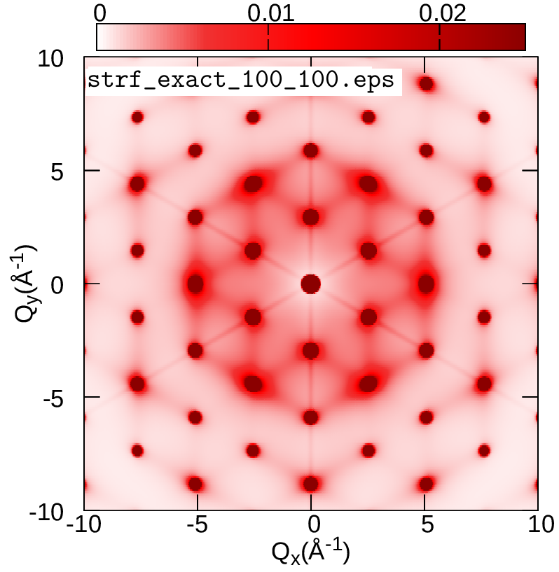
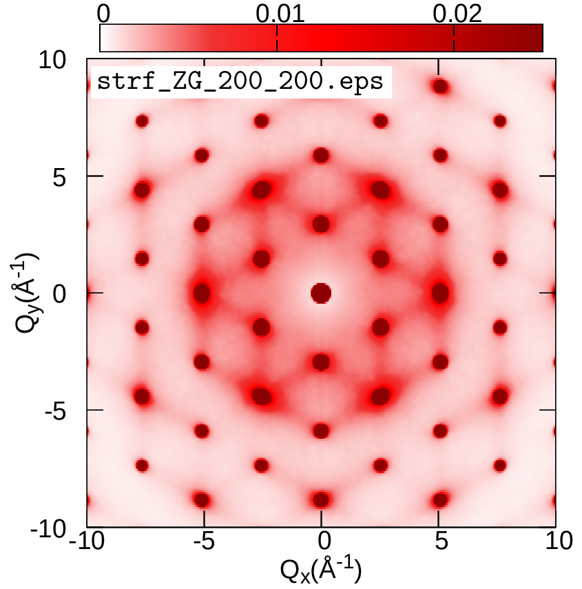
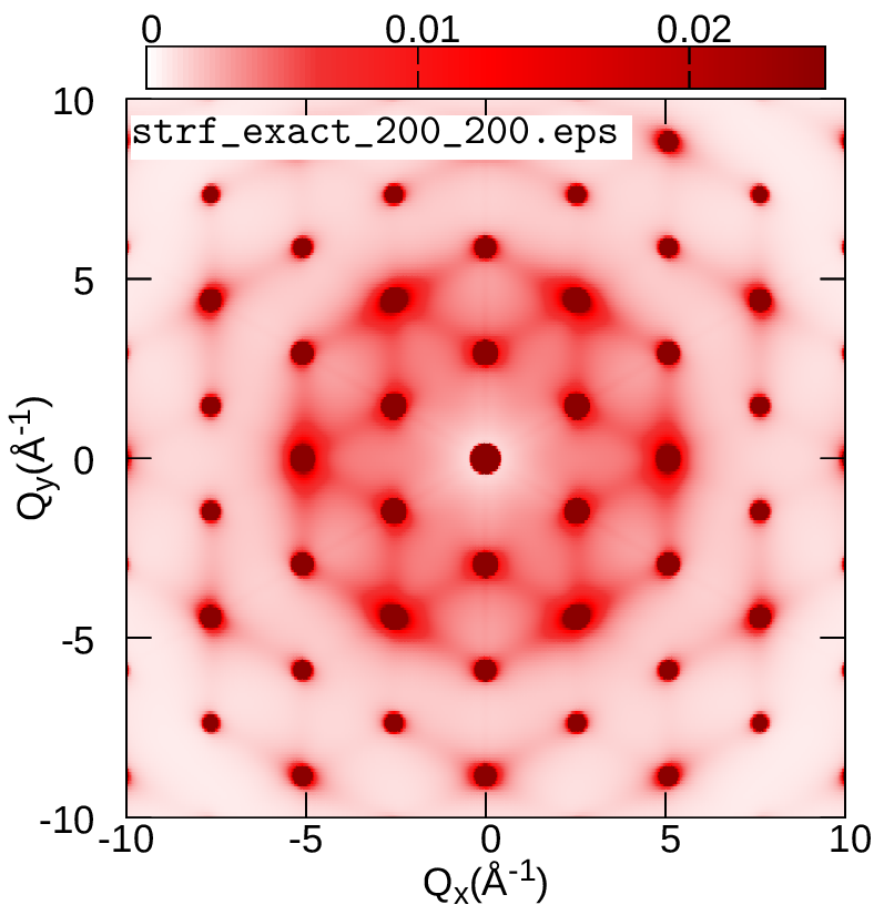
cd ../exact; gnuplot gp_pm3d.p; evince strf_exact_40_40.pdf
Your results should look like the plots below (left panel). We also add plots of the exact and ZG all-phonon structure maps using a \(100\times100\) and \(200\times200\) q-grid for Brillouin sampling. What happens to the ZG structure factor map as we approach the thermodynamic limit? Indeed, the choice of the order of signs is no longer important and the function \(E(\{S_{{\bf q} \nu}\})\) is minimized at the thermodynamic limit. Our calculations here also demonstrate the physical significance of the ZG configuration as the best collection of scatterers that reproduce the phonon-induced inelastic scattering.


Exercise 6
In this exercise we will learn how to perform phonon unfolding. This technique is useful to identify the effect on the phonons in the fundamental Brillouin zone when supercells are employed to accommodate disorder, defects, or any other perturbation that breaks the translational symmetry of the lattice. First, as a proof of concept, we will perform the perfect unfolding of the phonons calculated for a \(2\times2\times2\) silicon supercell; then we will show how to calculate the effect on the phonons when a \(2\times2\times2\) silicon supercell is doped by a phosphorous (P) atom.
Step 1
Go to exercise6, create workdir, and calculate the phonon dispersion of silicon in the unit cell using a \(2\times2\times2\) homogeneous \(\mathbf{q}\)-grid:
cd exercise6; cd workdir; cp -r ../inputs/unit_cell_222_grid/ .; cd unit_cell_222_grid/
$RUN_PW -nk 4 < si.scf.in > si.scf.out
$RUN_PH -nk 4 < si.ph.in > si.ph.out
$RUN_Q2R < q2r.in > q2r.out
$RUN_MATDYN < matdyn.in > matdyn.out
Input files are provided here:
si.scf.in
 &control
    calculation = 'scf'
    restart_mode = 'from_scratch',
    prefix = 'si',
    pseudo_dir = './',
    outdir='./'
 /
 &system
    ibrav = 2,
    celldm(1) = 10.20,
    nat =  2,
    ntyp = 1,
    ecutwfc = 30.0
 /
 &electrons
    diagonalization='david'
    mixing_mode = 'plain'
    mixing_beta = 0.7
    conv_thr = 1.0d-7
 /
ATOMIC_SPECIES
 Si  28.086  Si.pz-vbc.UPF
K_POINTS automatic
6 6 6 0 0 0
ATOMIC_POSITIONS {crystal}
 Si 0.00 0.00 0.00
 Si 0.25 0.25 0.25
/
si.ph.in
Phonons of Silicon
&inputph
   amass(1)= 28.0855,
   prefix = 'si'
   outdir = './'
   ldisp = .true.
   fildyn = 'si.dyn'
   tr2_ph = 1.0d-12
   nq1 = 2
   nq2 = 2
   nq3 = 2
/
q2r.in
&input
 fildyn='si.dyn', flfrc = 'si.222.fc'
/
matdyn.in
&input
    asr='simple', amass(1)=28.0855,
    flfrc='si.222.fc', fldyn='si.dyn.mat',
    flfrq='si.freq', fleig='si.dyn.eig', q_in_cryst_coord = .false.
    q_in_band_form = .true.
/
 9
 0         0         0      100
 0.75      0.75      0.0    1
 0.2500    1.0000    0.2500 100
 0.000     1         0.000  100
 0         0         0      100
 0.5000    0.5000    0.5000 100
 0         1         0      100
 0.5000    1.0000    0      100
 0.5000    0.5000    0.5000 100
/
Step 2
After the calculation is completed use :math:`plotband.x` of Quantum Espresso to obtain the phonon dispersion data as an a xmgr file.
$QE/plotband.x
Input file > si.freq
Reading    6 bands at    702 k-points
Range:    0.0000  510.0113eV  Emin, Emax, [firstk, lastk] > 0 600
high-symmetry point:  0.0000 0.0000 0.0000   x coordinate   0.0000
high-symmetry point:  0.7500 0.7500 0.0000   x coordinate   1.0607
...
high-symmetry point:  0.5000 0.5000 0.5000   x coordinate   5.3534
output file (gnuplot/xmgr) > si_ph_dispersion.xmgr
bands in gnuplot/xmgr format written to file si_ph_dispersion.xmgr
output file (ps) >
stopping ...
Step 3
Calculate the interatomic force constants of silicon using a \(2\times2\times2\) supercell and the \(\Gamma\)-point for the \(\mathbf{q}\)-grid.
cd ../; cp -r ../inputs/222_super/ .; cd 222_super
mpirun -np 48 $QE/pw.x -nk 4 < si.scf_222.in > si.scf_222.out
mpirun -np 48 $QE/ph.x -nk 4 < si.ph_222.in > si.ph_222.out
$RUN_Q2R < q2r.in > q2r.out
Input files are provided here:
si.scf_222.in
 &control
    calculation = 'scf'
    restart_mode = 'from_scratch',
    prefix = 'si',
    pseudo_dir = './',
    outdir='./'
 /
 &system
    ibrav = 2,
    celldm(1) = 20.40,
    nat =  16,
    ntyp = 1,
    ecutwfc = 20.0
 /
 &electrons
    diagonalization='david'
    mixing_mode = 'plain'
    mixing_beta = 0.7
    conv_thr = 1.0d-7
 /
ATOMIC_SPECIES
 Si  28.086  Si.pz-vbc.UPF
K_POINTS automatic
3 3 3 0 0 0
ATOMIC_POSITIONS (crystal)
Si   0.00000000   0.00000000   0.00000000
Si  -0.12500000   0.37500000  -0.12500000
Si   0.50000000   0.00000000   0.00000000
Si   0.37500000   0.37500000  -0.12500000
Si   0.00000000   0.50000000   0.00000000
Si  -0.12500000   0.87500000  -0.12500000
Si   0.50000000   0.50000000   0.00000000
Si   0.37500000   0.87500000  -0.12500000
Si   0.00000000   0.00000000   0.50000000
Si  -0.12500000   0.37500000   0.37500000
Si   0.50000000   0.00000000   0.50000000
Si   0.37500000   0.37500000   0.37500000
Si   0.00000000   0.50000000   0.50000000
Si  -0.12500000   0.87500000   0.37500000
Si   0.50000000   0.50000000   0.50000000
Si   0.37500000   0.87500000   0.37500000
si.ph.in
Phonons of Silicon
&inputph
   amass(1)= 28.0855,
   prefix = 'si'
   outdir = './'
   ldisp = .true.
   fildyn = 'si.dyn'
   tr2_ph = 1.0d-12
   nq1 = 1, nq2 = 1, nq3 = 1
/
q2r.in
&input
 fildyn='si.dyn', flfrc = 'si.222.fc'
/
Step 4
Perform phonon unfolding of the phonons of silicon calculated for a \(2\times2\times2\) supercell using ZG.x
mpirun -np 48 $QE/ZG.x -nk 48 < ZG_ph_unfold.in > ZG_ph_unfold.out
where the input file should look like:
ZG_ph_unfold.in
&input
    flfrc='si.222.fc',
    asr='simple', amass(1)=28.0855
    q_in_cryst_coord = .false., q_in_band_form = .true.
    ZG_conf = .false., ph_unfold = .true.
/
&phonon_unfold
     dim1 = 2, dim2 = 2, dim3 = 2
     ng1 = 14, ng2 = 14, ng3 = 14
     flfrq='frequencies.dat', flweights='unfold_weights.dat'
/
 9
   0.000000   0.000000   0.000000  74
   1.500000   1.500000   0.000000   1
   0.500000   2.000000   0.500000  24
   0.000000   2.000000   0.000000  70
   0.000000   0.000000   0.000000  60
   1.000000   1.000000   1.000000  60
   0.000000   2.000000   0.000000  34
   1.000000   2.000000   0.000000  50
   1.000000   1.000000   1.000000   1
/
Here, lines 2-4 contain standard inputs for a phonon dispersion calculation (as for matdyn.x). In line 5, we specify that we would like to use ZG.x for phonon unfolding (ph_unfold = .true.) and not to generate special displacements (ZG_conf = .false.). In the namelist &phonon_unfold we have: (i) dimX which are essentially the supercell dimensions, (ii) ng1, ng2, ng3 define the range of the reciprocal lattice vectors (and thus plane waves) that need to be employed for calculating the spectral weights. Check for convergence by increasing this number; already 14 is a tight value, (iii) flfrq is the name of the output file containing the frequencies for each band and \(\mathbf{Q}\)-point and (iv) flweights is the name of the output file containing the spectral weights for each band and \(\mathbf{Q}\)-point. At the end of the file we provide the high-symmetry path for which we would like to perform phonon unfolding. The input structure of path is in the same spirit with a matdyn.x calculation. As for the electron band structure unfolding, the coordinates of the \(\mathbf{Q}\)-points are obtained by multiplying the \(\mathbf{q}\) wavevectors (defining the fundamental Brillouin zone) with the dimensions of the supercell, i.e. if q \(= [ x \,\,\, y \,\,\, z]\) then Q \(= [ {\rm dim1} \times x \,\,\, {\rm dim2} \times y \,\,\, {\rm dim3} \times z]\).
Step 5
Now we have the phonon frequencies and their spectral weights, we can calculate the phonon spectral function using pp_spctrlfn.x. Convert first the raw data in frequencies.dat and unfold_weights.dat into a different format using plotband.x of QE (commands provided in bands.sh):
$QE/plotband.x unfold_weights.dat < spectral_weights.in > spectral_weights.out
$QE/plotband.x frequencies.dat < energies.in > energies.out
sed -i '/^\s*$/d' spectral_weights.dat # remove empty lines
sed -i '/^\s*$/d' energies.dat
paste energies.dat spectral_weights.dat > tmp
awk '{print $1,$2,$4}' tmp > energies_weights.dat; rm tmp
You have just generated energies_weights.dat file in a similar format to a “.gnu” file where the first column has the momentum-axis values, the second the phonon frequencies, and the third the spectral weights. Now proceed with the calculation of the spectral function:
mpirun -n 28 $QE/pp_spctrlfn.x -nk 28 < pp_spctrlfn.in > pp_spctrlfn.out
cp spectral_function.dat ../../gnuplot/spectral_function_222.dat
cd ../../gnuplot/; gnuplot gp_pm3d_222.p; evince ph_unfolding_perfect_222.pdf
where the input file should look like:
pp_spctrlfn.in
&input
  flin = 'energies_weights.dat'
  steps = 17952,
  ksteps = 300,
  esteps = 300,
  kmin = 0,
  kmax = 5.3534,
  emin =  -10
  emax = 550
  flspfn = 'spectral_function.dat'
/
Note: The description of the input flags is available at Exercise 2: Step 6.
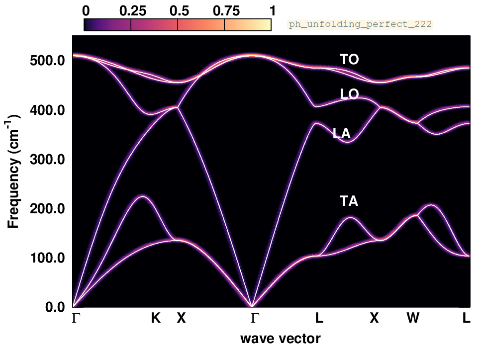
In this plot, the silicon phonon spectral function (color map) overlays with the phonon dispersion calculated in the unit cell, since the supercell is an exact periodic replica of the unit cell. One can also check the raw data in unfold_weights.dat, and observe that the weights of the phonon frequencies are either 1 or 0, making an one-to-one correspondence with the frequencies calculated in the unit cell.
Step 6
Now go to workdir, calculate the phonons of P-doped silicon, and perform phonon unfolding:
cd ../workdir/;cp -r ../inputs/222_super_P_doped .; cd 222_super_P_doped/
mpirun -np 48 $QE/pw.x -nk 4 < si.scf_222.in > si.scf_222.out
mpirun -np 48 $QE/ph.x -nk 4 < si.ph_222.in > si.ph_222.out
$RUN_Q2R < q2r.in > q2r.out
mpirun -np 48 $QE/ZG.x -nk 48 < ZG_ph_unfold.in > ZG_ph_unfold.out
Note: Here we replace one Si atom with a P atom and provide the relaxed structure. Due to the excess electron the system becomes metallic.
Here we provide all input files:
si.scf_222.in
 &control
    calculation = 'scf'
    restart_mode = 'from_scratch',
    prefix = 'si',
    pseudo_dir = './',
    outdir='./'
 /
 &system
    ibrav = 2,
    celldm(1) = 20.40,
    nat =  16,
    ntyp = 2,
    ecutwfc = 30.0
    occupations='smearing'
    degauss = 0.01
    nosym =.true.
 /
 &electrons
    diagonalization='david'
    mixing_mode = 'plain'
    mixing_beta = 0.7
    conv_thr = 1.0d-7
 /
ATOMIC_SPECIES
 Si  28.086  Si.pz-vbc.UPF
 P  30.974   P.pz-hgh.UPF
K_POINTS automatic
3 3 3 0 0 0
ATOMIC_POSITIONS (crystal)
P             0.0000000002       -0.0000000243        0.0000000412
Si           -0.1261235427        0.3783706126       -0.1261235364
Si            0.4983582216        0.0016417759        0.0016417825
Si            0.3751699490        0.3751699540       -0.1255098692
Si            0.0016417706        0.4983582252        0.0016417800
Si           -0.1261235463        0.8738764598       -0.1261235454
Si            0.4983582134        0.4983582133        0.0016417907
Si            0.3783706477        0.8738764517       -0.1261235465
Si            0.0016417985        0.0016418052        0.4983581945
Si           -0.1255098925        0.3751699883        0.3751699378
Si            0.4983582056        0.0016417944        0.4983582063
Si            0.3751699659        0.3751699770        0.3751699562
Si            0.0016417902        0.4983582115        0.4983582106
Si           -0.1261235587        0.8738764426        0.3783706794
Si            0.4999999969        0.5000000190        0.4999999746
Si            0.3751699807        0.8744900937        0.3751699437
/
si.ph_222.in
&inputph
   amass(1)= 28.0855,
   amass(2)= 30.974,
   prefix = 'si'
   outdir = './'
   ldisp = .true.
   fildyn = 'si.dyn'
   tr2_ph = 1.0d-12
   epsil = .false.
   nq1 = 1, nq2 = 1, nq3 = 1
/
q2r.in
&input
 fildyn='si.dyn', flfrc = 'si.222.fc'
/
ZG_ph_unfold.in
&input
    flfrc='si.222.fc',
    asr='simple', amass(1)=28.0855, amass(2)= 30.974
    q_in_cryst_coord = .false., q_in_band_form = .true.
    ZG_conf = .false.
    ph_unfold = .true.
/
&phonon_unfold
     dim1 = 2, dim2 = 2, dim3 = 2
     ng1 = 14, ng2 = 14, ng3 = 14
     flfrq='frequencies.dat', flweights='unfold_weights.dat'
/
 9
   0.000000   0.000000   0.000000  74
   1.500000   1.500000   0.000000   1
   0.500000   2.000000   0.500000  24
   0.000000   2.000000   0.000000  70
   0.000000   0.000000   0.000000  60
   1.000000   1.000000   1.000000  60
   0.000000   2.000000   0.000000  34
   1.000000   2.000000   0.000000  50
   1.000000   1.000000   1.000000   1
Step 7
The calculation should take around 4.5 minutes.
Now we have the phonon frequencies and their spectral weights, we can calculate the phonon spectral function using pp_spctrlfn.x as before. Convert first the raw data in frequencies.dat and unfold_weights.dat into a different format using plotband.x of QE (commands provided in bands.sh):
$QE/plotband.x unfold_weights.dat < spectral_weights.in > spectral_weights.out
$QE/plotband.x frequencies.dat < energies.in > energies.out
sed -i '/^\s*$/d' spectral_weights.dat # remove empty lines
sed -i '/^\s*$/d' energies.dat
paste energies.dat spectral_weights.dat > tmp
awk '{print $1,$2,$4}' tmp > energies_weights.dat; rm tmp
Step 8
Now proceed with the calculation of the spectral function:
mpirun -n 28 $QE/pp_spctrlfn.x -nk 28 < pp_spctrlfn.in > pp_spctrlfn.out
cp spectral_function.dat ../../gnuplot/spectral_function_222_P_doped.dat
cd ../../gnuplot/; gnuplot gp_pm3d_222_P_doped.p
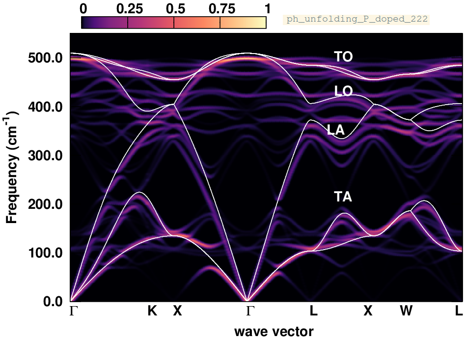
evince ph_unfolding_P_doped_222.pdf
where the input file pp_spctrlfn.in is the same as before.
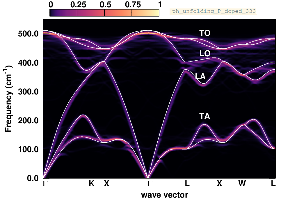
What are the changes in the phonon dispersion? Below we also provide the phonon spectral function calculated after replacing one Si atom with a P atom in a \(3\times3\times3\) supercell. Why are the changes less pronounced now?
APPENDIX / Exercise 2
In this section of the appendix we show how the band structure unfolding calculation can be broken down to one K-point at a time. This strategy is useful when the supercell size is large (larger than \(4\times4\times4\)) and the calculation requires a large amount of memory and storage space for the wavefunctions.
Step 1
Go to workdir/band_structure_unfolding of Exercise 1 and copy:
cp -r ../../../exercise1/workdir/ZG-0.00K-si.save/ .
cp ../../inputs/ZG-bands_333_0.00K.in ZG-bands_333_0.00K
cp ../../inputs/bands_unfold.in bands.in
In ZG-bands_333_0.00K apply the following modifications:
Set
calculation = 'bands'Delete the following lines containing information about the K-points:
K_POINTS crystal_b
2
0.000000 0.000000 0.000000 35
0.000000 1.500000 1.500000 1
At the bottom of the file add the following (after ZG atomic positions):
K_POINTS crystal_b
1
The file ZG-bands_333_0.00K should look like this:
ZG-bands_333_0.00K
&control
  calculation = 'bands'
  restart_mode = 'from_scratch'
  prefix = 'ZG-0.00K-si'
  pseudo_dir = './'
  outdir = './'
/
&system
  ibrav = 0
  nat =   54
  ntyp =    1
  nbnd = 135, nosym = .true., ecutwfc =  20.00
  occupations = 'smearing'
  smearing='gaussian',
  degauss=0.005d0
/
&electrons
  diagonalization = 'david'
  mixing_mode= 'plain'
  mixing_beta = 0.70
  conv_thr =   0.1D-06
/
ATOMIC_SPECIES
   Si   28.085 Si.pz-vbc.UPF
CELL_PARAMETERS {angstrom}
     -8.09641133      0.00000000      8.09641133
      0.00000000      8.09641133      8.09641133
     -8.09641133      8.09641133      0.00000000
ATOMIC_POSITIONS {angstrom}
...
K_POINTS crystal_b
1
Step 2
Prepare the K-point grid for band structure unfolding. To this aim run:
$QE/EPW/ZG/src/local/kpoints_band_str_unfold.x ! replace QE with path to QE dir
This script is designed to generate a list of K-points that will unfold back to the fundamental Brillouin zone. You will be asked to provide: (i) the number of high-symmetry k-points in the Brillouin zone of the unit-cell, (ii) their coordinates, (iii) their position along the \(\mathbf{k}\)-axis, (iv) the supercell size, and (v) whether you want to print every single K-point. For example:
Write number of high-symmetry kpts
2
 Write high-symmetry kpts (3 columns per row)
0.0 0.0 0.0
0.0 0.5 0.5
 Write x-positions of high-sym kpts
0.0
1.0
 Step is (default):  2.8571429E-02
 Supercell size (n * m * p) ?
3 3 3
 kpts to use for Supercell calculation:
   0.000000   0.000000   0.000000  35
   0.000000   1.500000   1.500000   1
 Write every single kpt? (0=no, 1=yes)
1
...
Note: for generating more K-points along the high-symmetry paths, you can increase the step value from the script: $QE/EPW/ZG/src/local/kpoints_band_str_unfold.f90. Pass all 35 K-points with their weights into a new file Kpoints.dat. Otherwise you can run:
cp ../../inputs/input_Kpoints.in .
$QE/EPW/ZG/src/local/kpoints_band_str_unfold.x \
  < input_Kpoints.in > Kpoints.dat
sed -i '1,9d' Kpoints.dat # deletes first 9 info lines from Kpoints.dat
Step 3
Run a band structure unfolding calculation.
cp ../../inputs/Kpoints.dat . # if you did not complete the previous action
cp ../../inputs/merge_files.sh .; ./merge_files.sh
Note: The script merge_files.sh will generate 35 input files si.333_ZG_bands_X.in to be used for a bands calculation for every single K-point. This strategy is the most efficient way to perform BSU in large supercells. Pass the following lines into a script and run:
# This script runs a bands calculation with "pw.x" and then performs
# band structure unfolding with "bands_unfold.x".
prefix=ZG-0.00K-si
i=1  # initial kpt index to calculate
f=35 # final kpt index to calculate
#
while [i -le $f ];do
    mkdir kpt_$i
    cd kpt_$i
#
    EXE=$QE/pw.x
    JNAME=ZG-bands_333_0.00K
#
    cp -r ../"$prefix".save .
    mv ../"$JNAME"_"$i".in .
    mpirun -n 14 $EXE  < "$JNAME"_"$i".in > "$JNAME"_"$i".out
#
    EXE=$QE/bands_unfold.x
    JNAME=bands
#
    cp ../"$JNAME".in .
    sed -i 's/tmp/'$i'/g'JNAME.in
    mpirun -n 14 $EXE  < "$JNAME".in > "$JNAME".out
#
    rm -r *wfc* "$prefix".save
    cd ../
    i=$((i+1))
done
Note: You can also copy the script from inputs, i.e. cp ../../inputs/script_bands.sh .
This script will generate the output directories kpt_X, containing the band energies files (bands01.dat) and spectral weights (spectral_weights01.dat) for each single K-point. The full calculation should take around 5 mins. Meanwhile you can check the progress of the calculation with ls -lrt and see how many kpt_X files have been generated so far. If kpt_1 exist, then check the outputs of bands01.dat and spectral_weights01.dat. The should contain the energies and spectral weights for K-point 1 (i.e. \(\Gamma\) here).
Step 4
Once energies and spectral weights for all K-points are calculated type:
cp ../../inputs/merge_kpts.sh .; ./merge_kpts.sh; cd all_kpts; ls
This will generate all_kpts directory and the new files bands01.dat and spectral_weights01.dat, containing the band energies, \(\varepsilon_{m {\bf K}}(T)\), and spectral weights, \(P_{m {\bf K}, {\bf k}} (T)\), for all K-points, respectively. Now you have all the ingredients to evaluate the spectral function as in Exercise 2.
Step 5
Now repeat all steps, starting from Step 6 of Exercise 2. (Note that you are one directory down, so modify accordingly; you might also need to modify steps in pp_spctrlfn.in to 4725)
APPENDIX / Exercise 3
In this section of the appendix we show how the calculation of temperature-dependent optical spectra can be broken down to one K-point at a time. This strategy is useful when the supercell size is large (larger than \(4\times4\times4\)) and the calculation requires a large amount of memory and storage space for the wavefunctions.
Step 1
First go to the directory exercise3, create your working directories and copy the input files:
cd ../../exercise3/; mkdir workdir; cd workdir; mkdir equil; mkdir ZG
cd equil
cp ../../inputs/equil/K_list.in .
cp ../../inputs/equil/epsilon.in .
cp ../../inputs/equil/epsi_av.sh .
cp -r ../../../exercise1/workdir/equil-si.save/ .
cp ../../../exercise2/workdir/equil-nscf_333.in equil-nscf_333
The file K_list.in contains the crystal coordinates of 200 randomly generated K-points with all weights set to 1.0 (we assign this weight, since we will perform calculations for each K-point separately, in a similar spirit with the BSU calculation). We use random K-points, instead of a uniform grid, to speed up convergence. In si.333_equil_nscf apply the following changes:
Add
nosym = .true.belownbnd = 135.Delete the information for the K-points:
K_POINTS crystal
2
0.000000 0.000000 0.000000 1
0.000000 1.260000 1.260000 1
and at the bottom of the file add the following:
K_POINTS crystal
1
Note: although we use the equilibrium structure we set nosym = .true. since random K-points are employed. The file equil-nscf_333 should look like this:
equil-nscf_333
&control
  calculation = 'nscf'
  restart_mode = 'from_scratch'
  prefix = 'equil-si'
  pseudo_dir = './'
  outdir = './'
/
&system
  ibrav = 0
  nat =   54
  ntyp =    1
  ecutwfc =  20.00
  nbnd = 135
  nosym = .true.
  occupations = 'fixed'
  smearing = 'gaussian'
  degauss =   0.0D+00
/
&electrons
  diagonalization = 'david'
  mixing_mode= 'plain'
  mixing_beta = 0.70
  conv_thr =   0.1D-06
/
ATOMIC_SPECIES
   Si   28.085 Si.pz-vbc.UPF
CELL_PARAMETERS {angstrom}
     -8.09641133      0.00000000      8.09641133
      0.00000000      8.09641133      8.09641133
     -8.09641133      8.09641133      0.00000000
ATOMIC_POSITIONS {angstrom}
   Si    0.00000000   0.00000000   0.00000000
   Si   -1.34940189   1.34940189   1.34940189
   Si   -2.69880378   0.00000000   2.69880378
...
K_POINTS crystal
1
Step 2
Run an optical spectrum calculation for silicon using the \(3\times3\times3\) equilibrium supercell and
30 random K-points. In the same spirit with the BSU calculation we calculate \(\epsilon_2(\omega)\) for every K-point using the following script:
prefix=equil-si
i=1  # initial kpt index to calculate
f=30 # final kpt index to calculate

while [i -le $f ];do
#
    JNAME=equil-nscf_333
    awk 'NR == '$i'' K_list.in > K_point.txt
    catJNAME K_point.txt > "$JNAME"_"$i".in
#
    mkdir kpt_$i
    cd kpt_$i
#
    EXE=$QE/pw.x
#
    cp -r ../"$prefix".save .
    mv ../"$JNAME"_"$i".in .
    mpirun -n 14 $EXE  < "$JNAME"_"$i".in > "$JNAME"_"$i".out
#
    EXE=$QE/epsilon_Gaus.x
    JNAME=epsilon
#
    cp ../"$JNAME".in .
    sed -i 's/tmp/'$i'/g'JNAME.in
    mpirun -n 14 $EXE  < "$JNAME".in > "$JNAME".out
#
    rm -r *wfc* "$prefix".save
    cd ../
    i=$((i+1))
done
Note: You can also copy the script from inputs, i.e. cp ../../inputs/equil/script_equil.sh .
This script will generate the output directories kpt_X, containing \(\epsilon_2(\omega)\) in the file epsi_equil-si.dat for each single K-point. The full calculation should take around 3 mins. Meanwhile you can check the progress of the calculation with ls -lrt and see how many kpt_X directories have been generated. If kpt_1 exist, then check the format of kpt_1/epsi_si_333_equil.dat. The first column is the energy grid, and the rest three represent \(\epsilon_2(\omega)\) along the three Cartesian directions.
Step 3
Once the calculation is completed run the script:
./epsi_av.sh
This script takes first the isotropic average of \(\epsilon_2(\omega)\) calculated for each K-point and then takes the average of \(\epsilon_2(\omega)\) over all K-points. The output file containing this data is epsi_si_333_equil_30.dat.
Note: epsi_av.sh takes the average over 30 K-points. You can modify this number using the variable m in the script.
Now copy the output file in the gnuplot directory using:
cp epsi_si_333_equil_30.dat ../../gnuplot/.
Step 4
Run an optical spectra calculation for silicon using the \(3\times3\times3\) ZG supercell following exactly the same procedure used for the equilibrium structure (as above); make sure now you use the file ZG-nscf_333_0.00K.in.