Polarons without supercells
07/29/2026
Note
Hands-on based on Quantum ESPRESSO v7.6 and EPW v6.1
Introduction
In this tutorial we will learn how to perform calculations of self-trapped polarons using the EPW code.
Prerequisites
This tutorial assumes that Quantum ESPRESSO and EPW have already been downloaded and compiled.
If you have not yet completed these steps,
please follow the Installation and setup tutorial before continuing.
The examples below also assume that the environment variables used to run the executables
(such as $QE, $RUN_PW, $RUN_PH, and $RUN_EPW) have been defined as described in the setup tutorial.
Note that variables defined with export only apply to the current terminal session.
If you compiled the code previously but are starting a new session,
you may need to redefine the run variables following the instructions in Defining run commands.
If the setup tutorial has been followed in the current session, the commands below should work directly in your terminal.
This tutorial builds on the standard DFT, DFPT, and electron-phonon interpolation workflow. If you are not already familiar with that workflow, we recommend completing the Interpolation of electron-phonon matrix elements tutorial first.
Download input files
The main input files are given explicitly throughout the tutorial. For convenience, they can also be downloaded here and extracted in your working directory before continuing. You may download them via the browser, or directly from the terminal:
pip install gdown
gdown https://drive.google.com/uc?id=19xZnYEgbYJHtXlYBXs58WSDAFVX9QogZ && tar -xzf tutorial05.tar.gz
cd tutorial05
Exercise 1: Small polarons
In this exercise, we will calculate the formation energy, lattice distortion, and wave function of a hole polaron in LiF.
Starting from ground-state DFT and DFPT calculations, we will construct the electron-phonon matrix elements in the Wannier representation, interpolate them onto fine momentum grids, and solve the self-consistent polaron equations with EPW.
Finally, we will analyze the polaron in real and reciprocal space and extrapolate its formation energy to the infinite-supercell limit.
Move to the exercise1 directory:
cd exercise1
and get the Li and F pseudopotential files from the Pseudo Dojo repository:
wget https://www.pseudo-dojo.org/pseudos/nc-sr-05_pbe_standard/Li.upf.gz && gunzip Li.upf.gz
wget https://www.pseudo-dojo.org/pseudos/nc-sr-05_pbe_standard/F.upf.gz && gunzip F.upf.gz
Step 1
Following the workflow introduced in the
Interpolation of electron-phonon matrix elements tutorial,
run a self-consistent calculation on an \(8\times8\times8\) \(\mathbf{k}\)-point grid using pw.x,
followed by a DFPT phonon calculation on a \(4\times4\times4\) \(\mathbf{q}\)-point grid using ph.x.
These calculations provide the quantities required for the subsequent electron-phonon and polaron calculations.
Use the following input files:
lif.scf.in
&control
    calculation     = 'scf'
    prefix          = 'lif'
    pseudo_dir      = './'
    outdir          = './'
    tprnfor         = .true.
    tstress         = .true.
/
&system
    ibrav           = 2
    celldm(1)       = 7.19084
    nat             = 2
    ntyp            = 2
    ecutwfc         = 60
/
&electrons
    conv_thr        = 1.0d-16
/
ATOMIC_SPECIES
 Li 6.941  Li.upf
 F 18.9984 F.upf
ATOMIC_POSITIONS crystal
 Li 0.0000 0.0000 0.0000
 F  0.5000 0.5000 0.5000
K_POINTS automatic
 8 8 8 0 0 0
lif.ph.in
&inputph
  prefix    = 'lif'
  outdir    = './'
  epsil     = .true.
  zeu       = .true.
  ldisp     = .true.
  fildyn    = 'lif.dyn'
  fildvscf  = 'dvscf'
  tr2_ph    =  1.0d-16,
  nq1       = 4,
  nq2       = 4,
  nq3       = 4
/
The calculations can be launched with the following commands:
$RUN_PW < lif.scf.in > lif.scf.out
$RUN_PH < lif.ph.in > lif.ph.out
Note: These coarse \(\mathbf{k}\)- and \(\mathbf{q}\)-point grids and the plane-wave expansion cutoff have been chosen to provide a reasonable balance between accuracy and computational cost. Fully converged calculations require denser coarse \(\mathbf{k}\) and \(\mathbf{q}\) grids, as well as a larger cutoff.
The keyword fildvscf tells ph.x to write the variations in the self-consistent potential
needed by EPW to compute the electron-phonon matrix elements
(see the PH input documentation).
As in the interpolation tutorial,
lif.dyn0 lists the 16 irreducible \(\mathbf{q}\) points,
while the lif.dynX and lif.dvscf1 files contain
the corresponding dynamical matrices and potential variations.
Step 2
Gather the .dyn and .dvscf files into a new save/ directory which EPW will read.
The files in _ph0/lif.phsave/ containing the displacement patterns are also needed.
This can be done using the pp.py Python script included in the EPW/bin distribution:
python3 $QE/../EPW/bin/pp.py
The script will ask you to enter the prefix of your calculation (in this case, lif):
Enter the prefix used for PH calculations (e.g. diam)
lif
Step 3
Run a non-self-consistent calculation on a full homogeneous \(4\times4\times4\) \(\mathbf{k}\)-point grid, then use EPW to construct the Wannier functions for the valence-band manifold and transform the electron-phonon matrix elements to the Wannier representation.
Begin with the following pw.x input file:
lif.nscf.in
&control
    calculation     = 'bands'
    prefix          = 'lif'
    pseudo_dir      = './'
    outdir          = './'
/
&system
    ibrav           = 2
    celldm(1)       = 7.19084
    nat             = 2
    ntyp            = 2
    ecutwfc         = 60
    nbnd            = 15
/
&electrons
    conv_thr        = 1.0d-16
/
ATOMIC_SPECIES
 Li 6.941  Li.upf
 F 18.9984 F.upf
ATOMIC_POSITIONS crystal
 Li 0.0000 0.0000 0.0000
 F  0.5000 0.5000 0.5000
K_POINTS crystal
64
  0.00000000  0.00000000  0.00000000  1.562500e-02
  0.00000000  0.00000000  0.25000000  1.562500e-02
  0.00000000  0.00000000  0.50000000  1.562500e-02
  0.00000000  0.00000000  0.75000000  1.562500e-02
  0.00000000  0.25000000  0.00000000  1.562500e-02
 ...
Note: The \(\mathbf{k}\)-point list shown above is abbreviated.
The downloaded lif.nscf.in file contains the complete grid, which can also be generated using the kmesh.pl script distributed with Wannier90:
$QE/../external/wannier90-3.1.0/utility/kmesh.pl 4 4 4
Next, prepare the EPW input file to calculate the electron-phonon matrix elements in the Wannier representation (lif.epw1.in):
lif.epw1.in
&inputepw
  prefix        = 'lif'
  outdir        = './'

  elph          = .true.
  epwwrite      = .true.

  lpolar        = .true.
  nbndsub       =  3
  dvscf_dir     = './save/'

  etf_mem       = 0

  bands_skipped = 'exclude_bands = 1:2, 6:15'
  wannierize    = .true.
  num_iter      = 500
  iprint        = 2

  proj(1)       = 'F:p'

  wannier_plot  = .true.
  wannier_plot_supercell = 4 4 4

  nk1           = 4
  nk2           = 4
  nk3           = 4
  nq1           = 4
  nq2           = 4
  nq3           = 4

  band_plot     = .true.
  filkf         = './path.kpt'
  filqf         = './path.kpt'
/
The auxiliary file path.kpt specifies the W-L-\(\Gamma\)-X-W-K path used by
filkf and filqf. It is included with the downloaded
tutorial files and is used again for the post-processing in Step 5.
The variable nbndsub selects three Wannier functions associated with the three isolated valence bands below the Fermi level. Consistent with their orbital character, proj sets the initial projections to three \(p\) orbitals centered on the F atom.
The calculations can be launched with the following commands:
$RUN_PW < lif.nscf.in > lif.nscf.out
$RUN_EPW < lif.epw1.in > lif.epw1.out
Step 4
Interpolate the electron-phonon matrix elements onto fine \(\mathbf{k}\)- and \(\mathbf{q}\)-point grids and solve the self-consistent polaron equations using the following input file:
lif.epw2.in
&inputepw
  prefix        = 'lif'
  outdir        = './'

  elph          = .true.
  epwread       = .true.
  lpolar        = .true.
  nbndsub       =  3
  dvscf_dir     = './save/'

  etf_mem       = 0

  wannierize    = .false.

  plrn              = .true.
  restart_plrn      = .false.
  type_plrn         = 1
  init_plrn         = 1
  init_sigma_plrn   = 2.0
  niter_plrn        = 500
  conv_thr_plrn     = 1E-4
  adapt_ethrdg_plrn = .true.
  ethrdg_plrn       = 1E-7

  nk1           = 4
  nk2           = 4
  nk3           = 4
  nq1           = 4
  nq2           = 4
  nq3           = 4

  nkf1          = 6
  nkf2          = 6
  nkf3          = 6
  nqf1          = 6
  nqf2          = 6
  nqf3          = 6
/
This calculation uses \(6\times6\times6\) fine \(\mathbf{k}\)- and \(\mathbf{q}\)-point grids.
The flags plrn = .true. and type_plrn = 1 activate the hole-polaron calculation.
For the initialization, init_plrn = 1 selects a Gaussian wave function, whose width is set to \(2.0~\mathrm{bohr}\) by init_sigma_plrn.
For convergence, conv_thr_plrn = 1E-4 requires the change in the atomic displacements between consecutive iterations to fall below \(10^{-4}~\mathrm{bohr}\).
Setting adapt_ethrdg_plrn = .true. progressively tightens the diagonalization threshold until it reaches ethrdg_plrn = 10^{-7} Ry.
Note: Since init_ethrdg_plrn and nethrdg_plrn are not specified, their default values are used.
Launch the calculation with:
$RUN_EPW < lif.epw2.in > lif.epw2.out
The evolution of the self-consistent solution is reported in lif.epw2.out.
Note: The excerpt below shows selected outer iterations. The repeated adaptive-diagonalization details are omitted.
Starting the self-consistent process
--------------------------------------------------------------------------------
 iter      Eigval/eV      Phonon/eV    Electron/eV   Formation/eV       Error/eV
    1     0.3413E+00    -0.1401E+00    -0.3333E+00     0.1932E+00     0.1308E+00
    2     0.1627E+01    -0.8474E+00    -0.7075E+00    -0.1399E+00     0.1891E+00
    3     0.2646E+01    -0.1655E+01    -0.8631E+00    -0.7918E+00     0.1424E+00
    4     0.2870E+01    -0.1865E+01    -0.8927E+00    -0.9728E+00     0.4726E-01
    5     0.2904E+01    -0.1899E+01    -0.8975E+00    -0.1001E+01     0.1318E-01
  ...
   10     0.2915E+01    -0.1907E+01    -0.8982E+00    -0.1009E+01     0.3527E-02
   11     0.2915E+01    -0.1907E+01    -0.8982E+00    -0.1009E+01     0.1028E-02
   12     0.2915E+01    -0.1907E+01    -0.8982E+00    -0.1009E+01     0.2974E-02
--------------------------------------------------------------------------------
End of self-consistent cycle
The energetics of the converged polaron solution are printed at the end:
      Eigenvalue (eV):        2.9153235
     Phonon part (eV):       -1.9072329
   Electron part (eV):        0.8982144
Formation Energy (eV):       -1.0090186
The electron and phonon contributions to the formation energy are defined in Eq. (49) in the polaron equations section of the Theory page. More details and further discussion can be found in Phys. Rev. B 99, 235139 (2019).
A quick inspection of the output files will show that several files have been written with the .plrn extension.
The most relevant output files for this exercise are Amp.plrn and dtau.plrn,
which contain the polaron wave function coefficients in the Wannier basis and the atomic displacements, respectively.
These files are needed to postprocess and analyze the polaron solution in more detail,
which will be done in the next step.
Step 5
Post-process the converged solution to visualize the polaron wave function and analyze its expansion coefficients in reciprocal space using the following input file:
lif.epw3.in
&inputepw
  prefix        = 'lif'
  outdir        = './'

  elph          = .true.
  epwread       = .true.
  lpolar        = .true.
  nbndsub       =  3
  dvscf_dir     = './save/'

  etf_mem       = 0

  wannierize    = .false.

  plrn              = .true.
  restart_plrn      = .true.
  type_plrn         = 1

  cal_psir_plrn     = .true.
  interp_Ank_plrn   = .true.
  interp_Bqu_plrn   = .true.
  filkf             = './path.kpt'
  filqf             = './path.kpt'

  nk1           = 4
  nk2           = 4
  nk3           = 4
  nq1           = 4
  nq2           = 4
  nq3           = 4

  nkf1          = 6
  nkf2          = 6
  nkf3          = 6
  nqf1          = 6
  nqf2          = 6
  nqf3          = 6
/
Setting restart_plrn = .true. skips the self-consistent cycle
and reads the converged wave function and displacements from Amp.plrn and dtau.plrn.
The flag cal_psir_plrn = .true. writes the real-space wave function to psir_plrn.xsf.
The flags interp_Ank_plrn and interp_Bqu_plrn
activate the interpolation of the wave-function and displacement coefficients, respectively.
The interpolation paths are read from the files specified by
filkf and filqf;
here, both use path.kpt along W-L-\(\Gamma\)-X-W-K.
Launch the post-processing calculation with:
$RUN_EPW < lif.epw3.in > lif.epw3.out
You can visualize psir_plrn.xsf with
VESTA:
VESTA psir_plrn.xsf
You should obtain something similar to this:
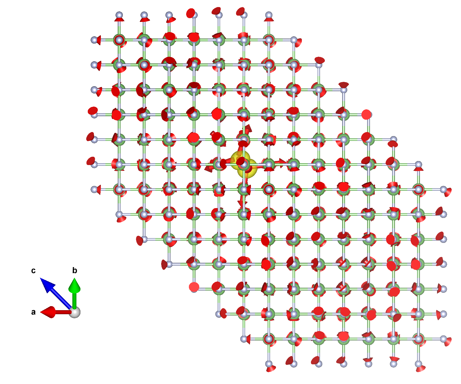
The wave function is shown as an isosurface, and the red arrows represent the atomic displacements. Note that the \(6\times6\times6\) momentum grid corresponds to a periodic \(6\times6\times6\) real-space supercell. The hole forms a small polaron localized within one unit cell, with a wave function concentrated on a single F site and exhibiting the characteristic shape of a \(p\) orbital.
The output files containing the interpolated coefficients are Ank.band.plrn and Bmat.band.plrn.
You can visualize your results by using, for example, the following script (plot_Ank.py):
plot_Ank.py
## Script to plot Ank coefficients
import matplotlib as mpl
mpl.use('Agg')
import matplotlib.pyplot as plt
import numpy as np
# change font on mathematical expressions on plots
mpl.rcParams['mathtext.fontset'] = 'cm'

# Read Ank file
ik, ibnd, ek0, ReAnk, ImAnk, AbsAnk = np.loadtxt('Ank.band.plrn',
                                            unpack=True, skiprows=1)

# Separate data in different bands
nbnd=int(max(ibnd))
maxik=int(max(ik))
Ak=np.zeros((maxik,nbnd))
ek=np.zeros((maxik,nbnd))
iklist=np.zeros((maxik,nbnd))
for i in range(maxik):
    for ibnd in range(nbnd):
        Ak[i][ibnd]=AbsAnk[i*nbnd+ibnd]
        ek[i][ibnd]=ek0[i*nbnd+ibnd]
        iklist[i][ibnd]=i

# Get vbm and bandwidth
vbm=max(ek[:,nbnd-1])
bandwidth=vbm-min(ek[:,0])

## Plot bands
f, ax = plt.subplots(figsize=(10,6))
ax.plot(iklist, ek, color='blue')

# Plot Ank
ax.scatter(iklist, ek, 100*Ak, color='gold', edgecolors='gray', alpha=0.8,
     label=r'$|A_{n\mathbf{k}}|$')

# Set tick params etc.
ax.set_ylim(-bandwidth-0.1*bandwidth,0.1*bandwidth)
ax.set_xlim((min(iklist[:,0]),max(iklist[:,0])))
ax.set_xticklabels([])
ax.tick_params(axis='x', color='black', labelsize='0', pad=0, length=0, width=0)
ax.tick_params(axis='y', color='black', labelsize='18', pad=5, length=5, width=1)
ax.set_ylabel(r'$E-E_{\mathrm{VBM}} ~ (\mathrm{eV})$', fontsize=25, labelpad=10)
ax.legend(loc='upper right', fontsize=25)

plt.savefig('Ank.pdf', bbox_inches='tight')
plt.savefig('Ank.png', dpi=200, bbox_inches='tight')
Note: The downloaded example files also include plot_Bqv.py for plotting the \(B_{\mathbf{q}\nu}\) coefficients. Like plot_Ank.py, it generates both PDF and PNG output.
Run the plotting scripts:
python3 plot_Ank.py
python3 plot_Bqv.py
This generates Ank.pdf and Ank.png for the wave-function coefficients, and Bqv.pdf and Bqv.png for the displacement coefficients.
Your figures should be similar to:
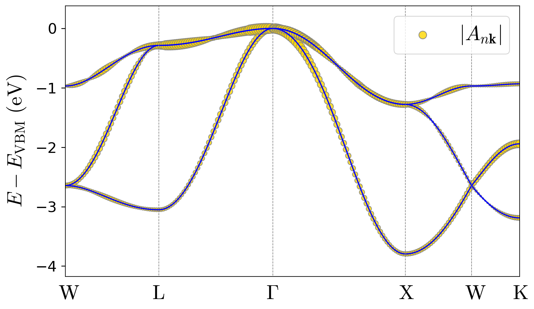
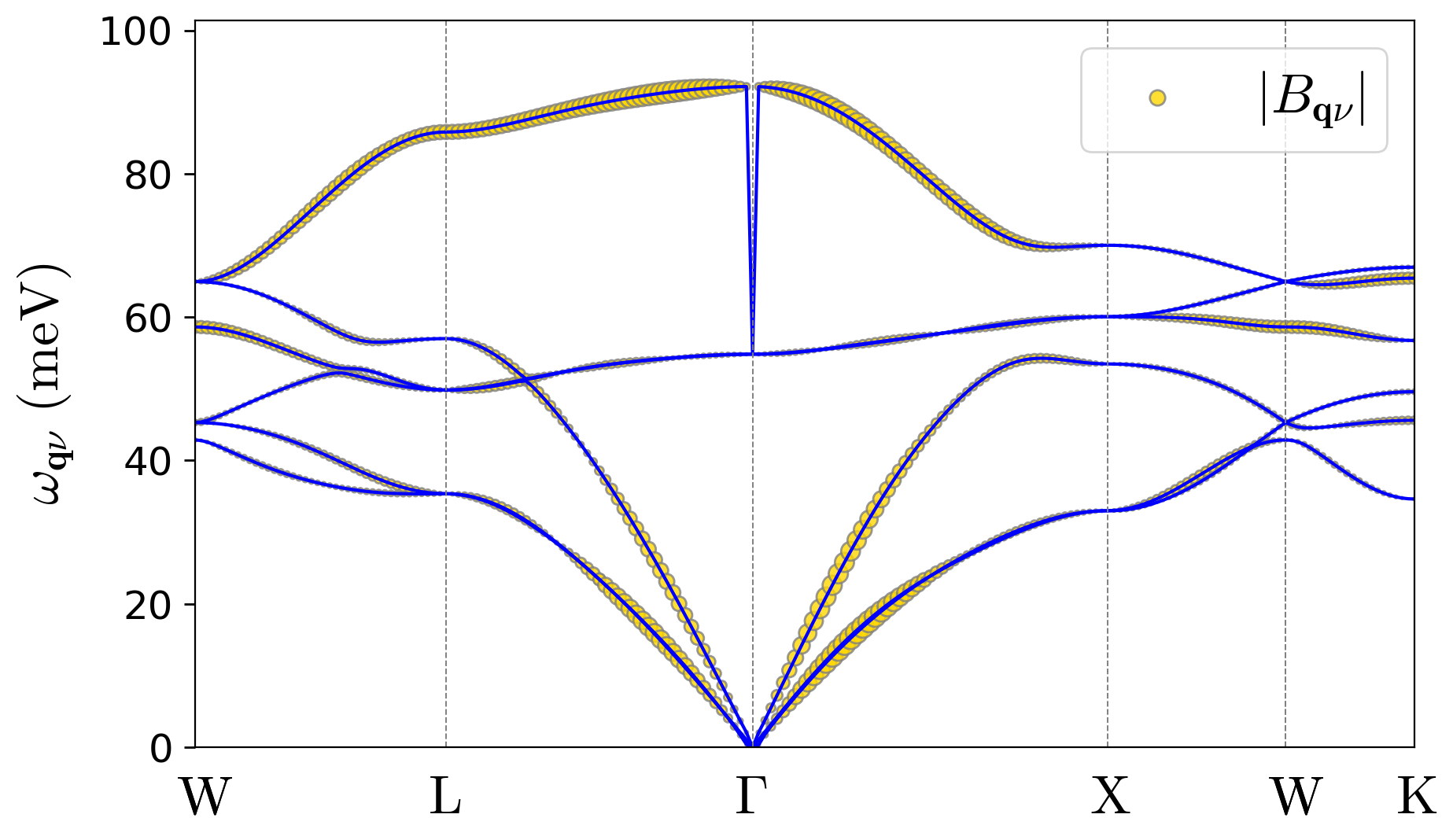
As you can observe in these results, due to the strongly localized nature of the hole polaron in LiF, its wave function coefficients in the Bloch basis are spread across the entire Brillouin zone. See the wave-function and displacement expansions in Eqs. (39) and (40) in the polaron equations section of the Theory page.
Step 6
Investigate the finite-supercell effects on the polaron formation energy defined in Eq. (49) in the polaron equations section of the Theory page, and extrapolate the results to the infinite-supercell limit.
A uniform \(N\times N\times N\) momentum grid corresponds to an \(N\times N\times N\) Born-von Kármán supercell, and the interaction between periodically repeated polarons introduces a supercell-size dependence in the formation energy.
The template lif.epw4.in can be obtained by copying the lif.epw2.in input
shown in Step 4. No manual changes are required because the script below creates
a separate input for each supercell size and updates all six fine-grid dimensions.
The prepared lif.epw4.in file is also included with the downloaded tutorial files.
cp lif.epw2.in lif.epw4.in
Then repeat the calculation for increasingly dense grids using the following script:
run_supercell_sizes.sh
#!/bin/bash
set -e

printf "#    nk      Eform\n" > E_vs_nk.dat

for nk in 8 10 12 14 16; do

  input="lif.epw4.${nk}.in"
  output="lif.epw4.${nk}.out"

  sed -e "s/^[[:space:]]*nkf1[[:space:]]*=.*/  nkf1 = ${nk}/" \
      -e "s/^[[:space:]]*nkf2[[:space:]]*=.*/  nkf2 = ${nk}/" \
      -e "s/^[[:space:]]*nkf3[[:space:]]*=.*/  nkf3 = ${nk}/" \
      -e "s/^[[:space:]]*nqf1[[:space:]]*=.*/  nqf1 = ${nk}/" \
      -e "s/^[[:space:]]*nqf2[[:space:]]*=.*/  nqf2 = ${nk}/" \
      -e "s/^[[:space:]]*nqf3[[:space:]]*=.*/  nqf3 = ${nk}/" \
      lif.epw4.in > "${input}"

  $RUN_EPW < "${input}" > "${output}"

  energy=$(awk '/Formation Energy \(eV\):/ {value=$NF} END {print value}' "${output}")
  printf "%6d %14s\n" "${nk}" "${energy}" >> E_vs_nk.dat
done
Run the script from the exercise1 directory:
bash run_supercell_sizes.sh
For each grid, the script updates the fine electron and phonon grid dimensions
(nkf1, nkf2, nkf3
and nqf1, nqf2, nqf3),
runs EPW using the previously defined RUN_EPW command,
and writes the final formation energy to E_vs_nk.dat:
#    nk      Eform
     8     -1.1935314
    10     -1.2961715
    12     -1.3522703
    14     -1.3912438
    16     -1.4165918
You can now plot the formation energy as a function of the inverse supercell size, \(L^{-1}\), where \(L^{3}\) is the supercell volume, and extrapolate to \(L^{-1}=0\) (infinite supercell size) using a linear fit to the three largest supercells:
plot_E_vs_nk.py
import matplotlib as mpl
mpl.use('Agg')
import matplotlib.pyplot as plt
from matplotlib.ticker import MultipleLocator
import numpy as np

# Read E vs nk
Nk, Eform = np.genfromtxt('E_vs_nk.dat', unpack=True)

# Set unit cell volume to convert Nk to inverse supercell size
ucell_volume = 92.9563
inverse_size = 1/(Nk*ucell_volume**(1/3))

# Start figure
fig, ax = plt.subplots(figsize=(12,8))

# Plot Eform
ax.scatter(inverse_size, Eform, s=50, marker='o',
     color='darkred', edgecolors='black')

# Fit the three largest supercells and extrapolate to infinite size
mf, bf = np.polyfit(inverse_size[-3:], Eform[-3:], 1)
xlist = np.linspace(inverse_size[-3], 0.0, 100)
print("Extrapolation to isolated polaron formation energy = ", "%.3f" % bf, "eV")
ax.plot(xlist, mf*xlist+bf, '--', color='gray')

# Set tick params etc.
ax.set_xlabel(r'Inverse supercell size ($\mathrm{bohr}^{-1}$)',fontsize=20)
ax.set_ylabel('Formation energy (eV)',fontsize=20, labelpad=5)
ax.tick_params(axis='x', color='black', labelsize='20', pad=5, length=5, width=2)
ax.tick_params(axis='y', color='black', labelsize='20', pad=5, length=5, width=2,
         right=True)
ax.yaxis.set_minor_locator(MultipleLocator(0.1))
ax.tick_params(axis='y', which='minor', color='black', labelsize='20', pad=5,
         length=3, width=1.2, right=True)
ax.set_xlim(0.0, np.max(inverse_size)+0.01)
ax.set_title('LiF hole polaron', fontsize=20)

plt.savefig("E_vs_nk.pdf", bbox_inches="tight")
plt.savefig("E_vs_nk.png", dpi=200, bbox_inches="tight")
Run the plotting script:
python3 plot_E_vs_nk.py
This generates E_vs_nk.pdf and E_vs_nk.png.
The resulting plot should be similar to:
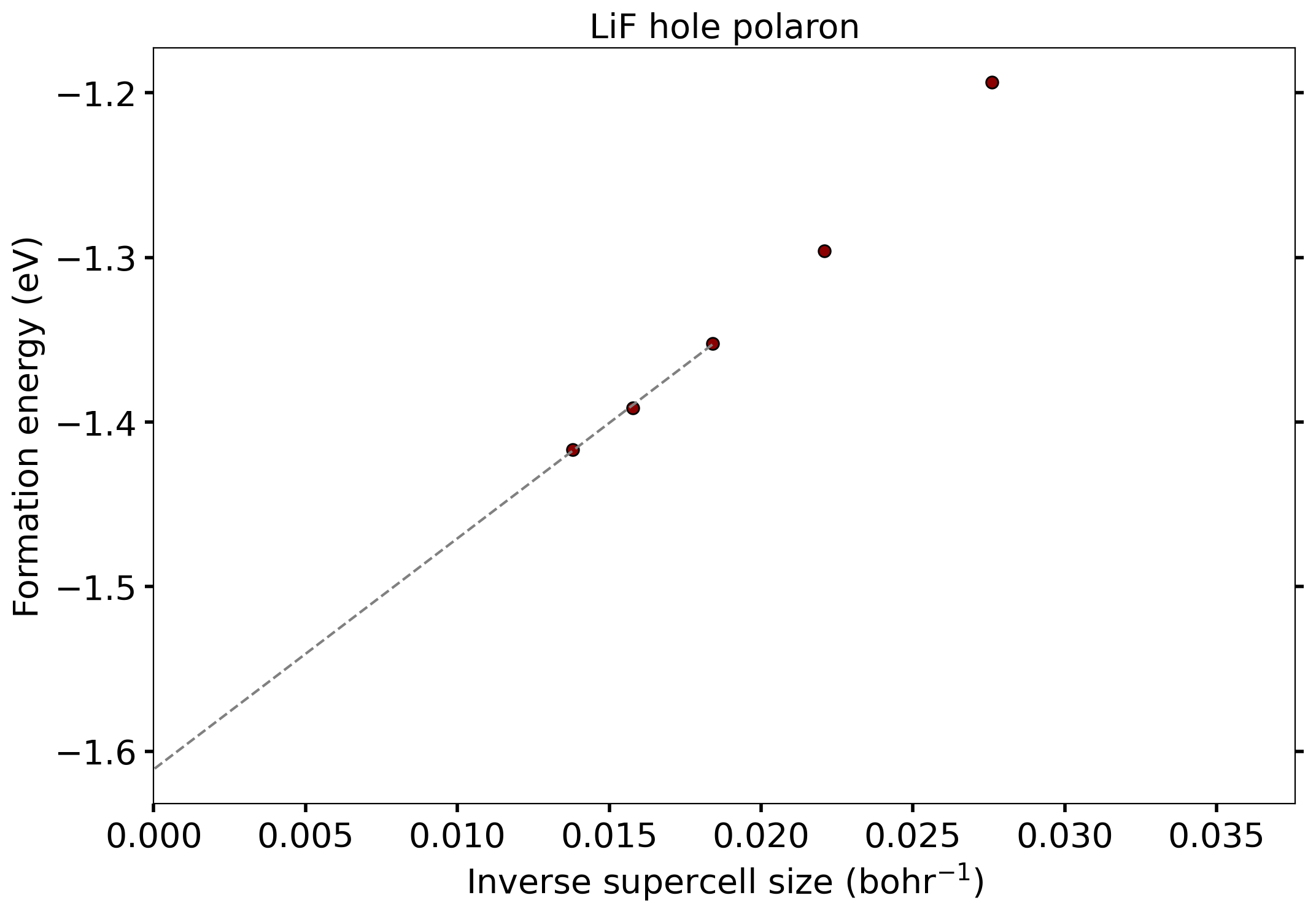
The fit to the three largest supercells gives an extrapolated formation energy of \(\Delta E_{f}=-1.611~\mathrm{eV}\) for the isolated hole polaron in LiF. Note that these illustrative calculations are not fully converged; see Phys. Rev. B 99, 235139 (2019) for converged calculation parameters.
Exercise 2: Large polarons
In this exercise, we will calculate the formation of electron polarons in LiF. The ground-state electronic structure, phonons, and perturbation potentials are unchanged from Exercise 1, so we will reuse those data and repeat only the EPW calculations for the conduction-band manifold.
Step 1
Move to the exercise2 directory and create symbolic links to the data generated in Exercise 1:
cd ../exercise2
ln -s ../exercise1/lif.save .
ln -s ../exercise1/save .
The same path.kpt high-symmetry path used in Exercise 1 is included in the
downloaded exercise2 directory.
If preparing the directory manually, it can
be copied from ../exercise1/path.kpt.
The lif.epw1.in input can be obtained by adapting the input of the same name from Step 3 of Exercise 1.
The key difference is that
nbndsub, bands_skipped, and proj
are configured to construct one Wannier function for the lowest conduction band
instead of the three valence-band Wannier functions used for the hole polaron.
A ready-to-run lif.epw1.in file is included with the downloaded tutorial files.
Calculate the electron-phonon matrix elements in the Wannier representation with:
$RUN_EPW < lif.epw1.in > lif.epw1.out
Step 2
Solve the electron-polaron equations for a series of increasingly large Born–von Kármán supercells.
The template lif.epw2.in can be obtained by adapting the input shown in Step 4 of Exercise 1:
it uses a single conduction band
and sets type_plrn = -1 to select an electron polaron calculation.
The initialization parameters are also adjusted for the more extended electron-polaron state.
The complete lif.epw2.in file is included with the downloaded tutorial files.
Use the following script to generate and run the inputs for \(6^3\) through \(16^3\) fine grids:
run_supercell_sizes.sh
#!/bin/bash
set -e

printf "#    nk      Eform\n" > E_vs_nk.dat

for nk in 6 8 10 12 14 16; do
  input="lif.epw2.${nk}.in"
  output="lif.epw2.${nk}.out"

  sed -e "s/^[[:space:]]*nkf1[[:space:]]*=.*/  nkf1 = ${nk}/" \
      -e "s/^[[:space:]]*nkf2[[:space:]]*=.*/  nkf2 = ${nk}/" \
      -e "s/^[[:space:]]*nkf3[[:space:]]*=.*/  nkf3 = ${nk}/" \
      -e "s/^[[:space:]]*nqf1[[:space:]]*=.*/  nqf1 = ${nk}/" \
      -e "s/^[[:space:]]*nqf2[[:space:]]*=.*/  nqf2 = ${nk}/" \
      -e "s/^[[:space:]]*nqf3[[:space:]]*=.*/  nqf3 = ${nk}/" \
      lif.epw2.in > "${input}"

  $RUN_EPW < "${input}" > "${output}"

  energy=$(awk '/Formation Energy \(eV\):/ {value=$NF} END {print value}' "${output}")
  printf "%6d %14s\n" "${nk}" "${energy}" >> E_vs_nk.dat
done
The ready-to-run run_supercell_sizes.sh script is also included in the
downloaded exercise2 directory.
Run the script from the exercise2 directory:
bash run_supercell_sizes.sh
For each grid, the script updates nkf1, nkf2, nkf3 and
nqf1, nqf2, nqf3, runs EPW using RUN_EPW, and writes the
formation energy defined in Eq. (49) in the
polaron equations section of the Theory page to
E_vs_nk.dat:
#    nk      Eform
     6     -0.0000000
     8      0.0167885
    10     -0.0638829
    12     -0.1154007
    14     -0.1507521
    16     -0.1765547
The formation energy becomes negative only when the supercell is large enough to accommodate the spatially extended electron-polaron wave function and its lattice distortion.
Step 3
Post-process the solution obtained on the \(16\times16\times16\) grid
to visualize the wave function and its reciprocal-space expansion coefficients.
The lif.epw3.in input can be obtained from lif.epw2.16.in
by setting
restart_plrn = .true. and enabling
cal_psir_plrn,
interp_Ank_plrn, and
interp_Bqu_plrn.
It also uses path.kpt through
filkf and filqf.
Setting step_wf_grid_plrn = 4 reduces
the density of the real-space grid used to evaluate the wave function,
lowering the cost of printing the wave function in this large supercell.
A ready-to-run lif.epw3.in file is included with the downloaded tutorial files.
Launch the post-processing calculation with:
$RUN_EPW < lif.epw3.in > lif.epw3.out
The plotting scripts can be obtained from Exercise 1:
cp ../exercise1/plot_Ank.py .
cp ../exercise1/plot_Bqv.py .
For the electron polaron, modify the energy range and label in plot_Ank.py to
reference the conduction-band minimum:
ax.set_ylim(-0.1*bandwidth, bandwidth+0.1*bandwidth)
ax.set_ylabel(r'$E-E_{\mathrm{CBM}} ~ (\mathrm{eV})$', fontsize=25, labelpad=10)
Ready-to-run versions of plot_Ank.py and plot_Bqv.py are included in the
downloaded exercise2 directory. Run them with:
python3 plot_Ank.py
python3 plot_Bqv.py
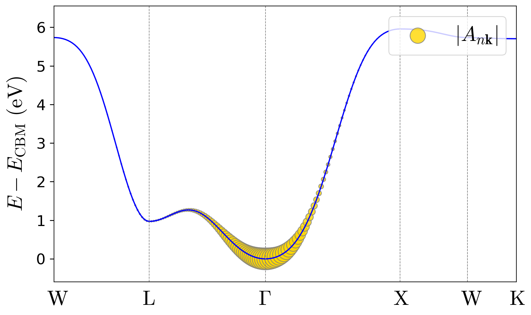
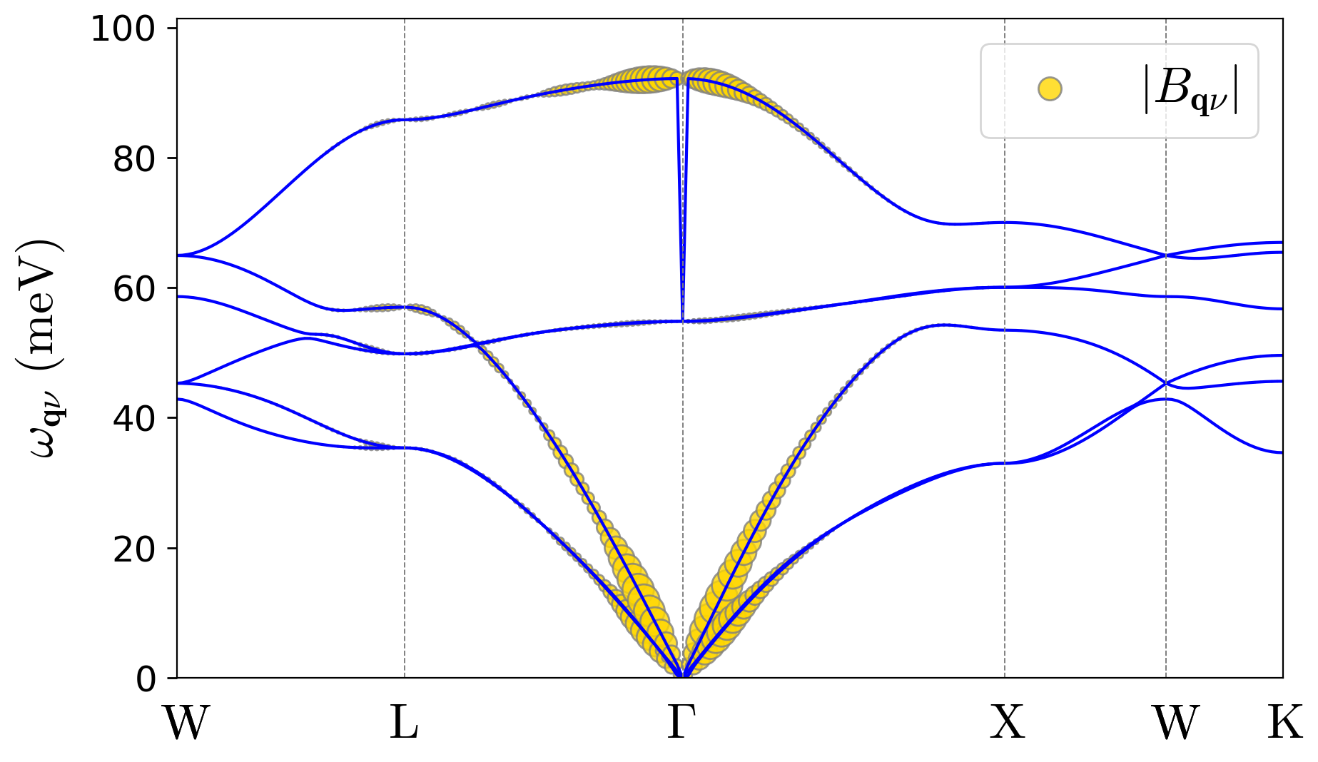
This generates Ank.pdf, Ank.png, Bqv.pdf, and Bqv.png. The
reciprocal-space coefficients should be similar to:
The real-space wave function can be visualized from psir_plrn.xsf using
VESTA:
VESTA psir_plrn.xsf
The result should be similar to:
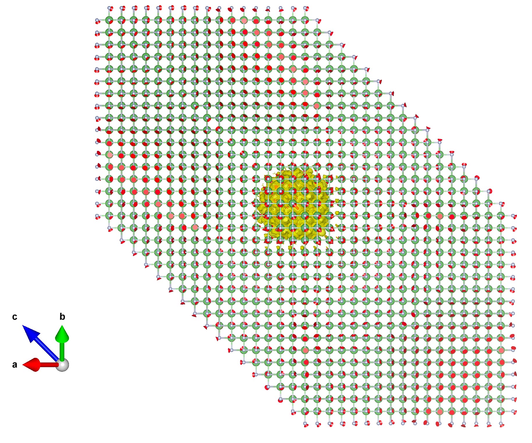
Unlike the localized hole polaron in Exercise 1, the electron forms a large polaron whose wave function extends over many unit cells. Correspondingly, the \(A_{n\mathbf{k}}\) coefficients are concentrated around the conduction-band minimum in reciprocal space, as expected from Eq. (39) in the polaron equations section of the Theory page.
Exercise 3: Non-diagonal supercells
In this exercise, we will calculate a hole polaron in rocksalt MgO and use a non-diagonal transformation matrix to represent a conventional cubic supercell. The direct- and reciprocal-lattice transformations are defined in Eqs. (47) and (48) in the polaron equations section of the Theory page.
Step 1
Move to the exercise3 directory:
cd ../exercise3
Download the Mg and O pseudopotentials from the Pseudo Dojo repository:
wget https://www.pseudo-dojo.org/pseudos/nc-sr-05_pbe_standard/Mg.upf.gz && gunzip Mg.upf.gz
wget https://www.pseudo-dojo.org/pseudos/nc-sr-05_pbe_standard/O.upf.gz && gunzip O.upf.gz
Perform the ground-state, phonon, and coarse-grid electron-phonon calculations.
The input files follow Steps 1–3 of
Exercise 1,
with the lattice, atomic species, pseudopotentials,
and Wannier manifold adapted to MgO.
Ready-to-run versions of
mgo.scf.in, mgo.ph.in, mgo.nscf.in, mgo.epw1.in,
and the auxiliary path.kpt file
are included with the download.
Here, nbndsub and proj select
the three O \(p\)-like valence-band Wannier functions relevant to the hole polaron.
Run the calculations with:
$RUN_PW < mgo.scf.in > mgo.scf.out
$RUN_PH < mgo.ph.in > mgo.ph.out
printf "mgo\n" | python3 $QE/../EPW/bin/pp.py > pp.out
$RUN_PW < mgo.nscf.in > mgo.nscf.out
$RUN_EPW < mgo.epw1.in > mgo.epw1.out
Step 2
Solve the self-consistent hole-polaron equations on homogeneous
\(6\times6\times6\) fine \(\mathbf{k}\)- and
\(\mathbf{q}\)-point grids
using mgo.epw2.in.
This input file can be obtained by adapting lif.epw2.in from
Step 4 of Exercise 1
to the MgO Wannier manifold.
A ready-to-run version is included with the downloaded tutorial files.
As in Exercise 1, type_plrn = 1 selects a hole-polaron calculation.
Launch the calculation with:
$RUN_EPW < mgo.epw2.in > mgo.epw2.out
Post-process the converged solution using mgo.epw3.in,
which is obtained from mgo.epw2.in
by enabling the same post-processing flags used in
Step 5 of Exercise 1.
The prepared file is included with the download.
$RUN_EPW < mgo.epw3.in > mgo.epw3.out
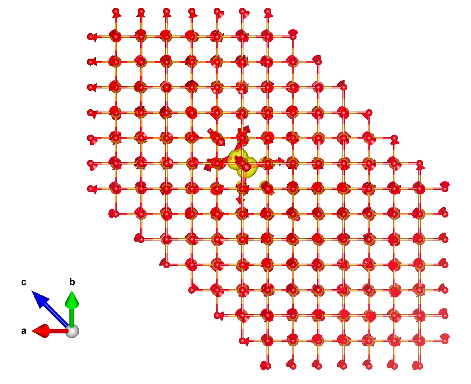
Visualize the resulting psir_plrn.xsf file with
VESTA:
VESTA psir_plrn.xsf
The result should be similar to:
Step 3
Repeat the hole-polaron calculation in a conventional \(4\times4\times4\)
cubic supercell using the non-diagonal transformation matrix in
mgo.epw4.in:
mgo.epw4.in
&inputepw
  prefix        = 'mgo'
  outdir        = './'

  elph          = .true.
  epwread       = .true.
  lpolar        = .true.
  nbndsub       =  3
  dvscf_dir     = './save/'

  etf_mem       = 0

  wannierize    = .false.

  plrn              = .true.
  restart_plrn      = .false.
  type_plrn         = 1
  init_plrn         = 1
  init_sigma_plrn   = 0.1
  niter_plrn        = 500
  conv_thr_plrn     = 1E-4
  ethrdg_plrn       = 1E-6

  nk1           = 4
  nk2           = 4
  nk3           = 4
  nq1           = 4
  nq2           = 4
  nq3           = 4

  scell_mat_plrn = .true.
  scell_mat(1, 1:3) = -4,  4, -4
  scell_mat(2, 1:3) = -4,  4,  4
  scell_mat(3, 1:3) =  4,  4, -4
/
scell_mat_plrn activates the non-diagonal-supercell construction, while scell_mat specifies the integer matrix \(S\) in Eq. (47) in the polaron equations section of the Theory page. For this matrix, \(|\det S|=256\), corresponding to 256 MgO primitive cells.
Note that, in this case,
the fine-grid dimensions are not specified through
nkf1, nkf2, nkf3 and nqf1, nqf2, nqf3.
EPW instead generates the compatible \(\mathbf{k}\)- and \(\mathbf{q}\)-point grids
from \(S\) and writes them to kgrid.scell.plrn.
The real-space lattice vectors are written to Rp.scell.plrn.
A ready-to-run mgo.epw4.in file is included with the downloaded tutorial files.
Launch the calculation with:
$RUN_EPW < mgo.epw4.in > mgo.epw4.out
The output reports the direct- and reciprocal-lattice transformations:
Supercell transformation activated (k), as=S*at
S(1, 1:3):   -4   4  -4
S(2, 1:3):   -4   4   4
S(3, 1:3):    4   4  -4
Transformed lattice vectors (alat units):
as(1, 1:3):     4.000000    0.000000    0.000000
as(2, 1:3):     0.000000    4.000000    0.000000
as(3, 1:3):     0.000000    0.000000    4.000000
Reciprocal lattice transformation matrix, Sbar = (S^{-1})^{t}:
Sbar(1, 1:3):    -0.125000    0.000000   -0.125000
Sbar(2, 1:3):     0.000000    0.125000    0.125000
Sbar(3, 1:3):     0.125000    0.125000    0.000000
Transformed reciprocal lattice vectors (2pi/alat units):
bs(1, 1:3):     0.250000    0.000000    0.000000
bs(2, 1:3):     0.000000    0.250000    0.000000
bs(3, 1:3):     0.000000    0.000000    0.250000

Number of unit cells within supercell:   256
Number of k-points needed:   256
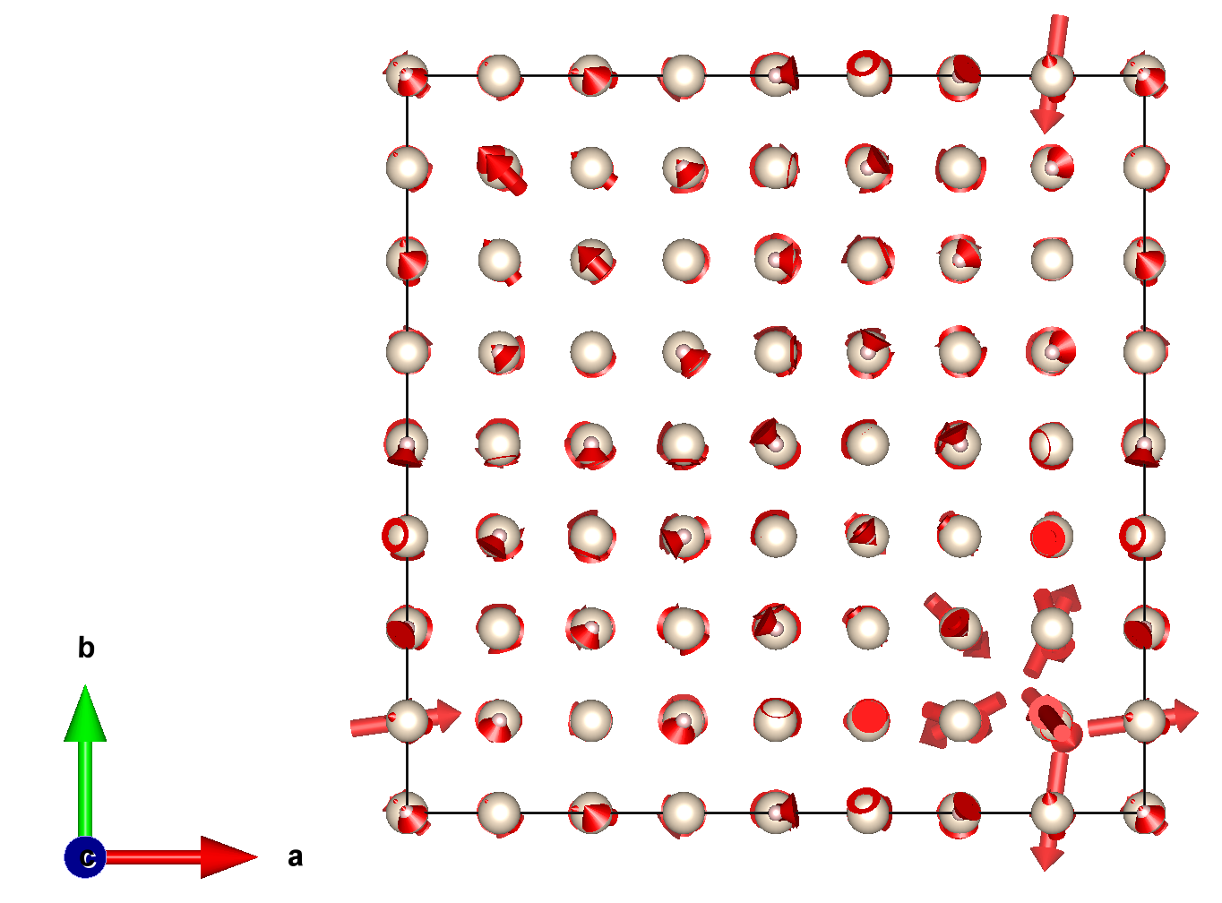
Visualize the final atomic displacements in dtau.plrn.xsf with VESTA:
VESTA dtau.plrn.xsf
The displacements of the hole polaron in the conventional cubic supercell of MgO should be similar to:
Exercise 4: Polaron energy landscapes
In this exercise, we calculate the adiabatic energy landscape for the nearest-neighbor hopping of a hole polaron in MgO. For each fixed atomic displacement configuration, EPW minimizes the energy with respect to the polaron wave function. The corresponding energy is given by Eq. (50) in the polaron equations section of the Theory page.
The input files and scripts for this exercise are included in the downloaded
exercise4 directory. We will reuse the interpolated electron–phonon data
and non-diagonal-supercell calculation from Exercise 3.
Step 1
The converged MgO hole-polaron displacements dtau.plrn obtained in
Step 3 of Exercise 3 provide the initial
configuration of the hopping path. Before continuing, check that the end of
exercise3/mgo.epw4.out reports a stable polaron solution:
--------------------------------------------------------------------------------
End of self-consistent cycle
      Eigenvalue (eV):        1.2681818
     Phonon part (eV):       -1.0823085
   Electron part (eV):        0.8967817
Formation Energy (eV):       -0.1855269
Move to the exercise4 directory, link the reusable EPW data, and copy the
converged displacement and supercell files:
cd ../exercise4
ln -s ../exercise3/mgo.save .
ln -s ../exercise3/save .
ln -s ../exercise3/*.fmt .
ln -s ../exercise3/mgo.epmatwp .
ln -s ../exercise3/mgo.ukk .
cp ../exercise3/dtau.plrn ../exercise3/Rp.scell.plrn .
The downloaded directory already contains mgo.epw5.in,
hopping_path.py, and plot_hopping_barrier.py.
Step 2
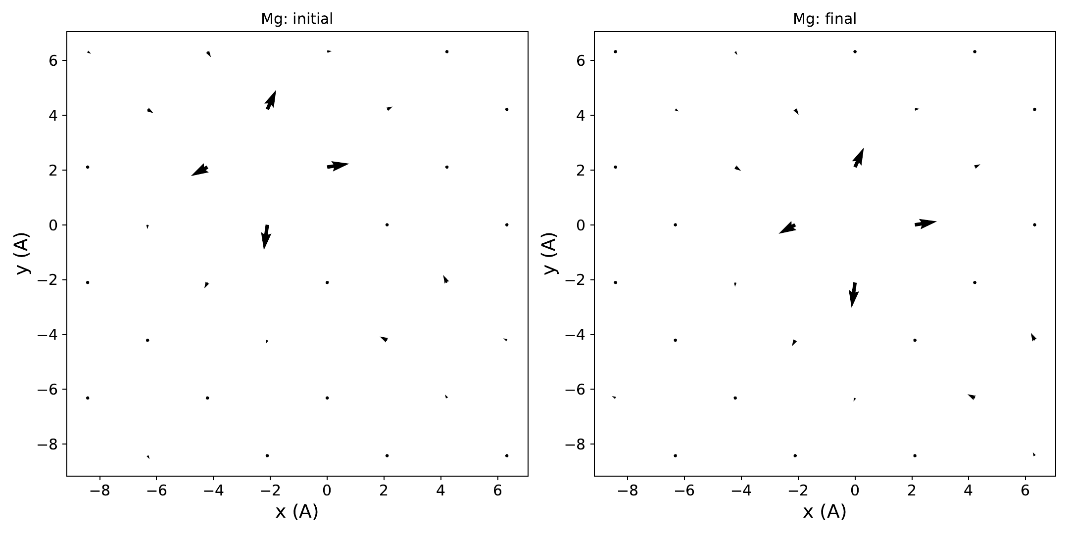
Construct a path between two equivalent polaron configurations on nearest-neighbor O sites.
The initial configuration is dtau.plrn;
the final configuration is obtained by translating this distortion
by one primitive cell along \([1,\bar{1},0]\).
The provided script (hopping_path.py)
linearly interpolates between them to generate 21 configurations:
python3 hopping_path.py
The script writes dtau_disp.plrn_1 through dtau_disp.plrn_21, which
will be read by EPW in the next step. It also writes
initial_final_displacements.pdf and
initial_final_displacements.png:
Step 3
Use mgo.epw5.in to evaluate the energy of each displacement
configuration:
mgo.epw5.in
&inputepw
  prefix        = 'mgo'
  outdir        = './'

  elph          = .true.
  epwread       = .true.
  lpolar        = .true.
  nbndsub       =  3
  dvscf_dir     = './save/'

  etf_mem       = 0

  wannierize    = .false.

  plrn              = .true.
  restart_plrn      = .false.
  type_plrn         = 1
  init_plrn         = 6
  init_ntau_plrn    = 21
  niter_plrn        = 1
  full_diagon_plrn  = .true.

  nk1           = 4
  nk2           = 4
  nk3           = 4
  nq1           = 4
  nq2           = 4
  nq3           = 4

  scell_mat_plrn = .true.
  scell_mat(1, 1:3) = -4,  4, -4
  scell_mat(2, 1:3) = -4,  4,  4
  scell_mat(3, 1:3) =  4,  4, -4
/
init_plrn is set to 6 to initialize the calculation from
fixed atomic displacement configurations.
init_ntau_plrn specifies the 21
dtau_disp.plrn_* files generated in
Step 2. Since only the electronic
degrees of freedom are minimized for each configuration,
niter_plrn is set to 1. This performs the single
diagonalization described in the
polaron equations section of the
Theory page, rather than a self-consistent update of
the displacements.
full_diagon_plrn = .true. selects the serial LAPACK diagonalization of
the effective polaron Hamiltonian. This is practical for the present small
grid and provides accurate eigenvalues, but is more computationally
expensive than the iterative solver.
The input is obtained from mgo.epw4.in by changing the initialization
and diagonalization variables shown above. A ready-to-run mgo.epw5.in
file is included with the downloaded tutorial files.
Launch the calculation with:
$RUN_EPW < mgo.epw5.in > mgo.epw5.out
For each configuration, mgo.epw5.out reports the eigenvalue, phonon and
electron contributions, and formation energy. The beginning of the output
should be similar to:
--------------------------------------------------------------------------------
 iter      Eigval/eV      Phonon/eV    Electron/eV   Formation/eV       Error/eV
    1     0.1271E+01    -0.1083E+01    -0.8952E+00    -0.1875E+00     0.2195E+00
      Eigenvalue (eV):        1.2707411
     Phonon part (eV):       -1.0826637
   Electron part (eV):        0.8951801
Formation Energy at this \dtau (eV):       -0.1880774
    1     0.1193E+01    -0.1008E+01    -0.8728E+00    -0.1352E+00     0.1089E-01
      Eigenvalue (eV):        1.1928718
     Phonon part (eV):       -1.0080353
   Electron part (eV):        0.8728328
Formation Energy at this \dtau (eV):       -0.1848365
    1     0.1117E+01    -0.9413E+00    -0.8489E+00    -0.9239E-01     0.1089E-01
      Eigenvalue (eV):        1.1166157
     Phonon part (eV):       -0.9412624
   Electron part (eV):        0.8488698
Formation Energy at this \dtau (eV):       -0.1753532
...
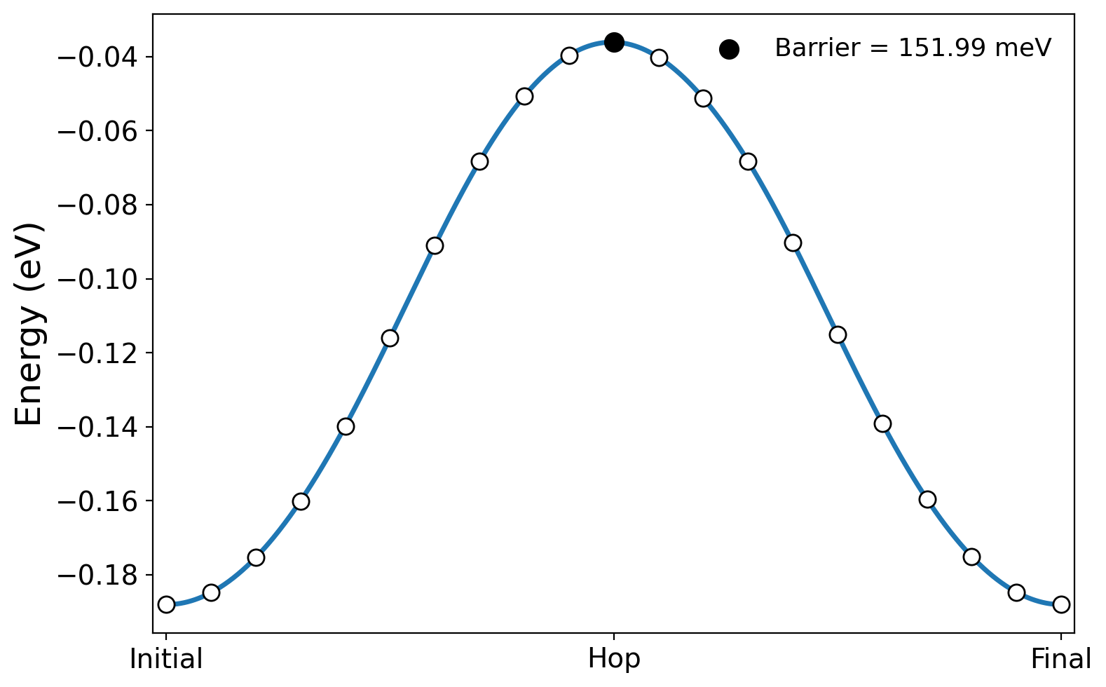
The energy rises as the polaron moves away from the initial site and falls as it approaches the equivalent final site. Plot the complete path with:
python3 plot_hopping_barrier.py
The script reads mgo.epw5.out, reports the barrier relative to the
initial configuration,
Hopping barrier relative to initial state: 151.99 meV
and writes hopping_barrier.pdf and hopping_barrier.png: