Superconducting properties
05/30/2026
Note
Hands-on based on QE-v7.5 and EPW-v6.0
In this tutorial we compute superconducting properties of two metals by solving the Migdal-Eliashberg equations with EPW: the isotropic case in fcc Pb (Exercise 1) and the anisotropic case in MgB2 (Exercise 2), where the gap equations are solved in three flavours – Fermi-surface restricted (FSR), full-bandwidth (FBW) with uniform Matsubara sampling, and full-bandwidth with sparse intermediate-representation (sparse-ir) Matsubara sampling. Theory background: Phys. Rev. B 87, 024505 (2013), npj Comput. Mater. 9, 1 (2023), Commun. Phys. 7, 33 (2024), Phys. Rev. B 110, 064505 (2024), and npj Comput. Mater. 11, 342 (2025).
Prerequisites
This tutorial assumes that Quantum ESPRESSO and EPW have already been downloaded and compiled.
If you have not yet completed these steps,
please follow the Installation and setup tutorial before continuing.
The examples below also assume that the environment variables used to run the executables
(such as $QE, $RUN_PW, $RUN_PH, and $RUN_EPW) have been defined as described in the setup tutorial.
Note that variables defined with export only apply to the current terminal session.
If you compiled the code previously but are starting a new session,
you may need to redefine the run variables following the instructions in Defining run commands.
If the setup tutorial has been followed in the current session, the commands below should work directly in your terminal.
This tutorial additionally requires the helper scripts pp.py and kmesh.pl (distributed with EPW and Wannier90), and norm-conserving pseudopotentials for Pb, Mg, and B in a shared pseudo/ directory (the bundle uses Pseudo Dojo ONCVPSP, scalar-relativistic, PBE).
The execution commands throughout the tutorial are written as $RUN_PW, $RUN_PH, $RUN_EPW, etc., without specifying parallelisation flags such as -nk.
Adjust the corresponding export RUN_*** definitions in the setup tutorial to match your machine (number of MPI ranks, -nk pools, MPI launcher).
Download input files
All input files are given explicitly throughout the tutorial. For convenience, the input files together with the pseudopotentials can also be downloaded here, and extracted in your working directory before continuing. You may download them via the browser, or directly from the terminal:
pip install gdown
gdown https://drive.google.com/uc?id=1teTRkfUHGnqCFlifWtC9TUCbHsxL9baj && tar -xzf tutorial04.tar.gz
cd tutorial04
Alternatively, fetch the pseudopotentials directly from the Pseudo Dojo repository into a pseudo/ directory:
mkdir -p pseudo && cd pseudo
wget https://www.pseudo-dojo.org/pseudos/nc-sr-05_pbe_standard/Pb.upf.gz && gunzip Pb.upf.gz
wget https://www.pseudo-dojo.org/pseudos/nc-sr-05_pbe_standard/Mg.upf.gz && gunzip Mg.upf.gz
wget https://www.pseudo-dojo.org/pseudos/nc-sr-05_pbe_standard/B.upf.gz  && gunzip B.upf.gz
cd ..
The sparse-ir object file ir_nlambda6_ndigit8.dat used in Exercise 2 is shipped with the bundle above in a separate sparse-ir/ directory; alternatively it can be regenerated with the Python sparse-ir package (see sparse-ir-fortran).
Exercise 1: Isotropic superconductivity in fcc Pb
We compute the superconducting gap, critical temperature, Eliashberg spectral function, and Fermi-surface nesting function of fcc Pb by solving the isotropic Migdal-Eliashberg equations. The exercise is self-contained: starting from a self-consistent calculation we obtain the harmonic phonons, Wannierise the electronic structure with EPW, and then exploit the new flag a2f_iso = .true. to evaluate \(\alpha^2 F(\omega)\) on the fly without writing the prefix.ephmat/ directory, substantially reducing the disk footprint.
Move to the Exercise 1 directory:
cd exercise1
Step 1
Run an SCF calculation on a homogeneous \(8\times8\times8\) \(\mathbf{k}\)-grid and a DFPT phonon calculation on a homogeneous \(6\times6\times6\) \(\mathbf{q}\)-grid:
cd phonon
$RUN_PW -in scf.in > scf.out
$RUN_PH -in ph.in  > ph.out
scf.in
&CONTROL
  calculation     = 'scf'
  prefix          = 'pb',
  restart_mode    = 'from_scratch'
  pseudo_dir      = '../../pseudo/',
  outdir          = './'
  tprnfor         = .true.
  tstress         = .true.
/
&SYSTEM
  ibrav           = 2,
  celldm(1)       = 9.508849701769328,
  nat             = 1,
  ntyp            = 1,
  ecutwfc         = 60.0
  occupations     = 'smearing',
  smearing        = 'm-p',
  degauss         = 0.04
/
&ELECTRONS
  diagonalization = 'david'
  mixing_mode     = 'plain'
  mixing_beta     = 0.7
  conv_thr        = 1.0d-10
/
ATOMIC_SPECIES
  Pb 207.2 Pb.upf
ATOMIC_POSITIONS {crystal}
  Pb 0.00 0.00 0.00
K_POINTS {automatic}
  8 8 8  0 0 0
ph.in
Lead
&INPUTPH
  prefix    = 'pb',
  outdir    = './'
  trans     = .true.,
  reduce_io = .true.
  fildyn    = 'pb.dyn',
  fildvscf  = 'dvscf'
  ldisp     = .true.,
  nq1 = 6,
  nq2 = 6,
  nq3 = 6,
  tr2_ph    = 1.0d-14,
  alpha_mix(1)  = 0.1
  alpha_mix(10) = 0.3
/
Step 2
Collect the .dyn, .dvscf, and patterns files into a new save/ directory using the helper script pp.py distributed with EPW:
python3 /path/to/EPW/bin/pp.py
Enter the prefix "pb" when prompted.
Step 3
Compute the inter-atomic force constants with q2r.x and the harmonic phonon dispersion and DOS with matdyn.x:
$RUN_Q2R     -in q2r.in     > q2r.out
$RUN_MATDYN  -in matdyn.in  > matdyn.out
$RUN_MATDYN  -in phdos.in   > phdos.out
q2r.in
&INPUT
  zasr   = 'crystal',
  fildyn = 'pb.dyn',
  flfrc  = 'pb.fc'
/
matdyn.in
&INPUT
  asr              = 'crystal',
  flfrc            = 'pb.fc',
  flfrq            = 'pb.freq',
  dos              = .false.
  q_in_band_form   = .true.,
  q_in_cryst_coord = .true.
/
  6
  0.000 0.000 0.000  50 ! \Gamma
  0.500 0.000 0.500  50 ! X
  0.500 0.250 0.750  50 ! W
  0.500 0.500 0.500  50 ! L
  0.000 0.000 0.000  50 ! \Gamma
  0.375 0.375 0.750  1  ! K
phdos.in
&INPUT
  asr   = 'crystal',
  flfrc = 'pb.fc',
  flfrq = 'pb.freq',
  dos   = .true.,
  fldos = 'pb.phdos',
  nk1=24, nk2=24, nk3=24
/
Step 4
Move to the epw directory and run a non-self-consistent calculation on a \(6\times6\times6\) \(\Gamma\)-centred \(\mathbf{k}\)-grid, followed by the EPW Wannierisation:
cd ../epw
$RUN_PW  -in nscf.in > nscf.out
$RUN_EPW -in epw1.in > epw1.out
epw1.in
&INPUTEPW
  prefix      = 'pb',
  amass(1)    = 207.2
  outdir      = './'
  dvscf_dir   = '../phonon/save'

  elph        = .true.

  epbwrite    = .true.
  epbread     = .false.
  epwwrite    = .true.
  epwread     = .false.
  etf_mem     = 0
  epw_memdist = .true.

  lifc        = .true.
  asr_typ     = 'crystal'

  nbndsub     = 4
  bands_skipped = 'exclude_bands = 1:5'

  wannierize  = .true.
  num_iter    = 3000
  iprint      = 2
  dis_froz_max = 16.5
  dis_froz_min = -1.0
  proj(1)     = 'Pb:sp3'
  wdata(1)  = 'begin kpoint_path'
  wdata(2)  = 'G  0.00000  0.00000  0.00000 X  0.00000  0.50000  0.50000'
  wdata(3)  = 'X  0.00000  0.50000  0.50000 W -0.25000  0.50000  0.25000'
  wdata(4)  = 'W -0.25000  0.50000  0.25000 K -0.37500  0.37500  0.00000'
  wdata(5)  = 'K -0.37500  0.37500  0.00000 G  0.00000  0.00000  0.00000'
  wdata(6)  = 'G  0.00000  0.00000  0.00000 L  0.00000  0.50000  0.00000'
  wdata(7)  = 'L  0.00000  0.50000  0.00000 U  0.00000  0.62500  0.37500'
  wdata(8)  = 'U  0.00000  0.62500  0.37500 W -0.25000  0.50000  0.25000'
  wdata(9)  = 'W -0.25000  0.50000  0.25000 L  0.00000  0.50000  0.00000'
  wdata(10) = 'L  0.00000  0.50000  0.00000 K -0.37500  0.37500  0.00000'
  wdata(11) = 'end kpoint_path'
  wdata(12) = 'bands_plot = .true.'
  wdata(13) = 'bands_plot_format = gnuplot'
  wdata(14) = 'guiding_centres = .true.'
  wdata(15) = 'dis_num_iter      = 2000'
  wdata(16) = 'num_print_cycles  = 10'
  wdata(17) = 'dis_mix_ratio     = 0.5'
  wdata(18) = 'conv_window = 3'
  wdata(19) = 'write_hr = .true.'
  wdata(20) = 'use_ws_distance = .true.'

  nk1 = 6
  nk2 = 6
  nk3 = 6
  nq1 = 6
  nq2 = 6
  nq3 = 6

  nkf1 = 1
  nkf2 = 1
  nkf3 = 1
  nqf1 = 1
  nqf2 = 1
  nqf3 = 1
/
EPW writes pb.epmatwp, pb.ukk, crystal.fmt, epwdata.fmt, vmedata.fmt (or dmedata.fmt), and wigner.fmt, which encode the electron-phonon matrix elements in the Wannier representation. These files are reused by all subsequent EPW steps.
Step 5
Stay in the epw directory and run a single EPW job that solves the isotropic Migdal-Eliashberg equations on the imaginary axis, performs Pade and iterative analytic continuation, and computes \(\alpha^2 F(\omega)\) on the fly. The Wannier files written by Step 4 (pb.epmatwp, pb.ukk, *.fmt) are read in directly via epwread = .true.:
$RUN_EPW -in epw2.in > epw2.out
epw2.in
&INPUTEPW
  prefix      = 'pb',
  amass(1)    = 207.2
  outdir      = './'
  dvscf_dir   = '../phonon/save'

  etf_mem     = 0
  epw_memdist = .true.

  elph        = .true.
  epwread     = .true.
  epwwrite    = .false.

  lifc        = .true.
  asr_typ     = 'crystal'

  wannierize  = .false.
  nbndsub     = 4
  bands_skipped = 'exclude_bands = 1:5'

  fsthick     = 0.2     ! Fermi window thickness [eV]
  degaussw    = 0.05    ! electronic smearing [eV]
  degaussq    = 0.15    ! phonon smearing [meV]

  a2f_iso     = .true.  ! compute alpha^2 F on the fly
  eliashberg  = .true.

  liso  = .true.        ! isotropic Migdal-Eliashberg
  limag = .true.        ! imaginary-axis equations
  lpade = .true.        ! Pade continuation
  lacon = .true.        ! iterative real-axis continuation

  nsiter         = 500
  npade          = 12
  conv_thr_iaxis = 1.0d-4
  conv_thr_racon = 1.0d-4

  wscut = 0.1           ! Matsubara cutoff [eV]
  muc   = 0.1           ! effective Coulomb parameter

  temps = 0.3 0.9 1.5 2.1 2.7 3.3 4.0 4.5 4.6 4.7 4.8 4.9 5.0 5.1 5.2 5.3 5.4 5.5 5.6 5.7 5.8 5.9 6.0

  nk1 = 6
  nk2 = 6
  nk3 = 6
  nq1 = 6
  nq2 = 6
  nq3 = 6

  mp_mesh_k = .true.
  nkf1 = 48
  nkf2 = 48
  nkf3 = 48
  nqf1 = 24
  nqf2 = 24
  nqf3 = 24
/
Note. a2f_iso = .true. sets ephwrite = .false. and laniso = .false.; only the isotropic case is supported.
With these flags EPW
Fourier-transforms the electron-phonon matrix elements from the coarse \(6\times6\times6\) \(\mathbf{k}\)-grid and \(6\times6\times6\) \(\mathbf{q}\)-grid to the dense \(48\times48\times48\) \(\mathbf{k}\)-grid and \(24\times24\times24\) \(\mathbf{q}\)-grid.
Computes \(\alpha^2 F(\omega)\) on the fly during the iteration and writes
pb.a2fandpb.a2f_proj.Solves the isotropic Migdal-Eliashberg equations on the imaginary axis self-consistently at each temperature in temps.
Performs Pade (lpade
= .true.) and iterative (lacon= .true.) analytic continuation to the real frequency axis.
Expected output:
===================================================================
Solve isotropic Eliashberg equations
===================================================================
Electron-phonon coupling strength =    1.1583616

Estimated Tc using McMillan expression =   4.3678 K for muc =   0.1000
Estimated Tc using Allen-Dynes modified McMillan expression =   4.7481 K
Estimated Tc using SISSO machine learning model =   4.8882 K
Estimated w_log =   4.3952 meV
Estimated BCS superconducting gap using McMillan Tc =   0.6624 meV

Actual number of frequency points (     1) =    616 for uniform sampling

temp(  1) =      0.30000 K

Solve isotropic Eliashberg equations on imaginary-axis

Total number of frequency points nsiw(     1) =    616
   iter      ethr          znormi      deltai [meV]
     1   3.252901E+00   2.093070E+00   0.780552E+000
     2   1.393039E-01   2.087572E+00   0.824011E+000
     ...
     8   6.434965E-05   2.071107E+00   0.922654E+000
Convergence was reached in nsiter =      8
EPW writes one set of output files per temperature; XX stands for the temperature tag (e.g. 000.30 for \(T = 0.3\) K):
pb.a2f– isotropic Eliashberg spectral function \(\alpha^2 F(\omega)\) (col 2) and cumulative coupling \(\lambda(\omega)\) (col 3) as a function of frequency \(\omega\) (col 1, in meV).pb.a2f_proj– the same spectral function resolved by atomic contributions.pb.imag_iso_XX– Matsubara frequency, renormalisation \(Z\), and gap \(\Delta\) (eV).pb.pade_iso_XX– real-axis frequency, real and imaginary parts of \(Z\) and \(\Delta\) (eV) from Pade continuation.pb.acon_iso_XX– same layout aspb.pade_iso_XX, from the iterative continuation.
Combine the harmonic phonon dispersion (Step 3) and the spectral function pb.a2f (Step 5) in a single overview plot with the following gnuplot script:
plot_phbands.gnu
set terminal pngcairo color enhanced font "Times,30" fontscale 1.0 size 1400,900 lw 2
set out "fig1.png"
set multiplot
set border lw 1.75

ymin = 0
ymax = 10
set yrange [ymin:ymax]
set ytics 2
set mytics 2
set ytics scale 1.2,0.8
set xtics scale 1.2,0.8

# Panel 1: Phonon dispersion (left)
set lmargin at screen 0.10
set rmargin at screen 0.50
set bmargin at screen 0.18
set tmargin at screen 0.95
set ylabel "{/Symbol w} (meV)" offset 1,0
set xtics ("{/Symbol G}" 0, "X" 1, "W" 1.5, "L" 2.2071, "{/Symbol G}" 3.0731, "K" 4.1338) nomirror
set xrange [0:4.1338]
set arrow 1 from 1, graph 0 to 1, graph 1 nohead lw 1.5 dt 2
set arrow 2 from 1.5, graph 0 to 1.5, graph 1 nohead lw 1.5 dt 2
set arrow 3 from 2.2071, graph 0 to 2.2071, graph 1 nohead lw 1.5 dt 2
set arrow 4 from 3.0731, graph 0 to 3.0731, graph 1 nohead lw 1.5 dt 2
unset key
plot "../phonon/pb.freq.gp" u 1:($2/8.06554) w l lw 2 lt -1, \
     "../phonon/pb.freq.gp" u 1:($3/8.06554) w l lw 2 lt -1, \
     "../phonon/pb.freq.gp" u 1:($4/8.06554) w l lw 2 lt -1

# Panel 2: Phonon DOS (middle)
set lmargin at screen 0.54
set rmargin at screen 0.74
set bmargin at screen 0.18
set tmargin at screen 0.95
unset arrow
unset ylabel
set format y ""
set xlabel "PhDOS\n(states/meV)"
set xrange [0:1.0]
unset xtics
set xtics 0.4 nomirror
set xtics scale 1.2,0.8
set mxtics 2
unset key
plot "../phonon/pb.dos" u ($2*8.06554):($1/8.06554) w l lw 2.5 lt -1

# Panel 3: a2f and lambda (right)
set lmargin at screen 0.77
set rmargin at screen 0.97
set bmargin at screen 0.18
set tmargin at screen 0.95
set format y ""
set ytics nomirror
set xlabel "{/Symbol a}^2F({/Symbol w}), {/Symbol l}({/Symbol w})"
set xrange [0:1.25]
unset xtics
set xtics 0.5 nomirror
set xtics scale 1.2,0.8
set mxtics 2
set key at graph 0.95, 0.05 bottom right reverse Left samplen 2 spacing 1.3 nobox
plot "pb.a2f" u 2:1 w l lw 2.5 lt -1 title "{/Symbol a}^2F", \
     "pb.a2f" u 3:1 w l lw 2.5 lt 1 lc rgb "red" dt (6,3) title "{/Symbol l}"

unset multiplot
unset out
Run the script with gnuplot:
gnuplot plot_phbands.gnu
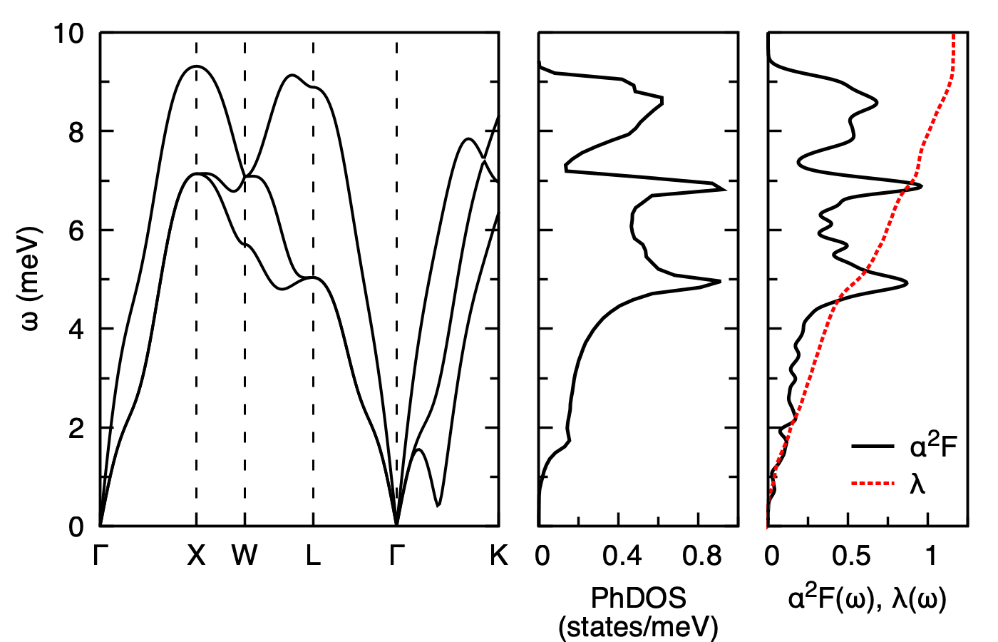
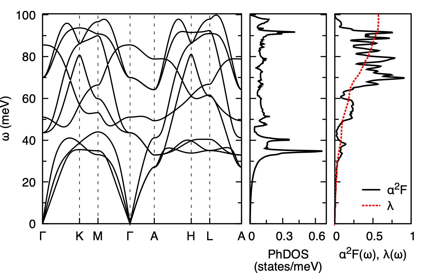
Calculated phonon dispersion (left), phonon density of states (middle), and Eliashberg spectral function \(\alpha^2 F(\omega)\) with cumulative electron-phonon coupling \(\lambda(\omega)\) (right) of fcc Pb. The total isotropic coupling \(\lambda \approx 1.16\) is read off as the asymptotic value of \(\lambda(\omega)\).
Plot the gap on the imaginary and real axes at \(T = 0.3\) K with the following gnuplot script:
plot_gap_conv.gnu
set terminal pngcairo color enhanced font "Times,28" fontscale 1.2 size 2000,850 lw 2
set out "fig2.png"
set multiplot
set border lw 2
set key spacing 1.5
set ytics scale 1.2,0.8
set xtics scale 1.2,0.8

set lmargin screen 0.09
set rmargin screen 0.47
set tmargin screen 0.94
set bmargin screen 0.20
set ylabel "{/=34 {/Symbol D} (meV)}" offset 0.5, 0
set xlabel "{/=34 i{/Symbol w} (meV)}" offset 0, -0.2
set tics font ",32"
set xtics 20
set ytics 0.2
set mxtics 2
set mytics 2
set key font ",24"
set xrange [0:60]
set yrange [-0.25:1.0]
plot "pb.imag_iso_000.30" u ($1*1000):($3*1000) w l lw 2 lt 1 lc rgb "black" notitle

reset
set border lw 2
set lmargin screen 0.56
set rmargin screen 0.96
set tmargin screen 0.94
set bmargin screen 0.20
set ylabel "{/=34 {/Symbol D} (meV)}" offset 1, 0
set xlabel "{/=34 {/Symbol w} (meV)}" offset 0, -0.2
set tics font ",32"
set xtics 20
set ytics 1.0
set mxtics 2
set mytics 2
set key font ",24"
set xrange [0:60]
set yrange [-1.8:2.5]
set key at graph 0.95, 0.9
plot "pb.pade_iso_000.30" u ($1*1000):($4*1000) w l lw 2 dt 1 lc rgb "black" title "Re({/Symbol D})-Pade approx.", \
     "pb.pade_iso_000.30" u ($1*1000):($5*1000) w l lw 2 dt 2 lc rgb "red"   title "Im({/Symbol D})-Pade approx.", \
     "pb.acon_iso_000.30" u ($1*1000):($4*1000) w l lw 2 dt 4 lc rgb "green" title "Re({/Symbol D})-analytic cont.", \
     "pb.acon_iso_000.30" u ($1*1000):($5*1000) w l lw 2 dt 3 lc rgb "blue"  title "Im({/Symbol D})-analytic cont."

unset multiplot
reset
Run the script with gnuplot:
gnuplot plot_gap_conv.gnu
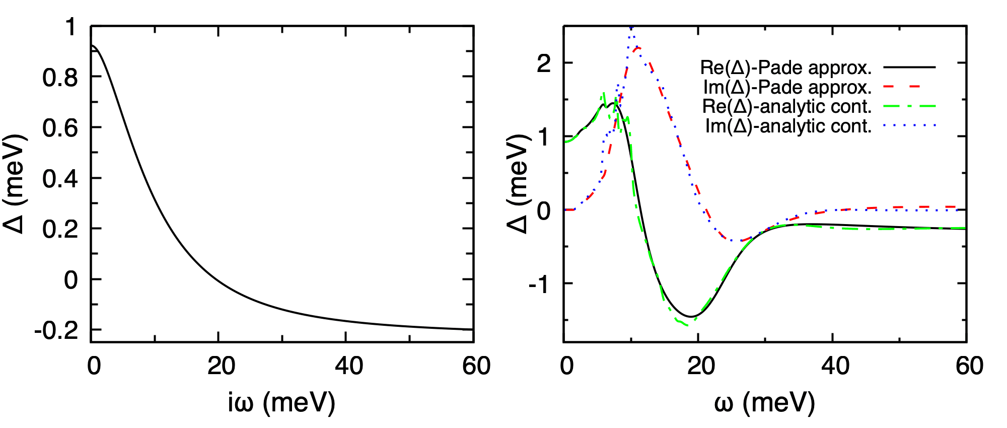
Superconducting gap of fcc Pb at \(T = 0.3\) K. Left: imaginary-axis \(\Delta(i\omega_n)\) from pb.imag_iso_000.30. Right: real-axis \(\Delta(\omega)\) from pb.pade_iso_000.30 (Pade) and pb.acon_iso_000.30 (iterative continuation).
Step 6
Extract the leading-edge gap \(\Delta_0(T)\) at each temperature with the helper scripts: script_gap0_imag reads the smallest Matsubara frequency from every pb.imag_iso_XX file; script_gap0_pade and script_gap0_acon do the same for the real-axis files.
script_gap0_imag
#!/bin/tcsh
awk 'FNR==2 {print FILENAME,$0}' pb.imag_iso_* | awk '{print $1 "   " $4*1000}' > pb.imag_iso_gap0
sed -i.bak 's/pb.imag_iso_//' pb.imag_iso_gap0 && rm pb.imag_iso_gap0.bak
script_gap0_pade
#!/bin/tcsh
awk 'FNR==2 {print FILENAME,$0}' pb.pade_iso_* | awk '{print $1 "   " $5*1000}' > pb.pade_iso_gap0
sed -i.bak 's/pb.pade_iso_//' pb.pade_iso_gap0 && rm pb.pade_iso_gap0.bak
script_gap0_acon
#!/bin/tcsh
awk 'FNR==2 {print FILENAME,$0}' pb.acon_iso_* | awk '{print $1 "   " $5*1000}' > pb.acon_iso_gap0
sed -i.bak 's/pb.acon_iso_//' pb.acon_iso_gap0 && rm pb.acon_iso_gap0.bak
Plot the imaginary-axis gap with plot_gap_imag.gnu and the comparison of all three continuations with plot_gap_all.gnu:
plot_gap_imag.gnu
set terminal pngcairo color enhanced font "Times,28" fontscale 1.2 size 1000,850 lw 2
set border lw 2
set key spacing 1.5
set ytics scale 1.6,0.9
set xtics scale 1.6,0.9
set ylabel "{/=34 {/Symbol D}_0 (meV)}" offset 0.8, 0
set xlabel "{/=34 Temperature (K)}" offset 0, -0.2
set lmargin screen 0.18
set rmargin screen 0.96
set tmargin screen 0.94
set bmargin screen 0.20
set tics font ",32"
set xtics 1
set ytics 0.4
set mxtics 2
set mytics 4
set key font ",24"
set xrange [0:6]
set yrange [0:1.2]
set out "fig3.png"
set key at graph 0.9, 0.9
plot "pb.imag_iso_gap0" with lp pt 7 ps 1.5 lw 2.5 dt 2 lc rgb "blue" notitle
reset
plot_gap_all.gnu
set terminal pngcairo color enhanced font "Times,28" fontscale 1.2 size 1000,850 lw 2
set border lw 2
set key spacing 1.5
set ytics scale 1.6,0.9
set xtics scale 1.6,0.9
set ylabel "{/=34 {/Symbol D}_0 (meV)}" offset 0.8, 0
set xlabel "{/=34 Temperature (K)}" offset 0, -0.2
set lmargin screen 0.18
set rmargin screen 0.96
set tmargin screen 0.94
set bmargin screen 0.20
set tics font ",32"
set xtics 1
set ytics 0.4
set mxtics 2
set mytics 4
set key font ",18"
set xrange [0:6]
set yrange [0:1.2]
set out "fig4.png"
set key at graph 0.96, 0.95
plot \
  "pb.imag_iso_gap0" using 1:($2 < 1.2 ? $2 : 1/0) with lp pt 7 ps 1.5 lw 2.5 dt 2 lc rgb "blue"  title "{/Symbol D}(i{/Symbol w}_{min}) (lowest Matsubara freq.)", \
  "pb.pade_iso_gap0"                              with lp pt 7 ps 1.5 lw 2.5 dt 2 lc rgb "black" title "{/Symbol D}({/Symbol w}=0) (Pade approx.)", \
  "pb.acon_iso_gap0"                              with lp pt 7 ps 1.5 lw 2.5 dt 2 lc rgb "red"   title "{/Symbol D}({/Symbol w}=0) (analytic cont.)"
reset
Run the helper scripts and gnuplot scripts:
./script_gap0_imag
./script_gap0_pade
./script_gap0_acon
gnuplot plot_gap_imag.gnu
gnuplot plot_gap_all.gnu
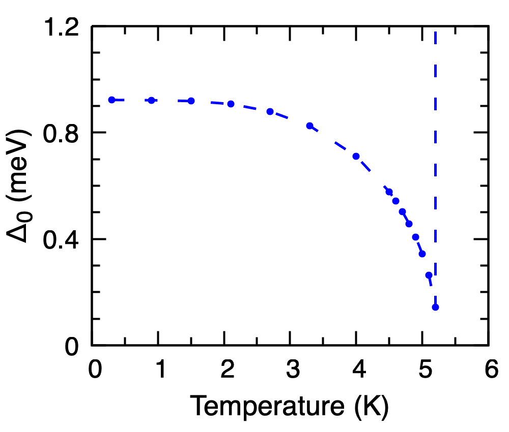
Calculated isotropic gap \(\Delta_0(T)\) of Pb on the imaginary axis as a function of temperature, taken from the lowest Matsubara frequency of each pb.imag_iso_XX file. The vertical dashed line marks the temperature at which the gap closes (\(T_c \approx 5.2\) K).
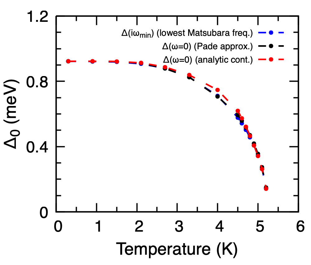
Comparison of the temperature-dependent gap of Pb from the imaginary axis (lowest Matsubara frequency), the Pade continuation (\(\Delta(\omega = 0)\)), and the iterative analytic continuation. The three curves should agree within the precision of the continuation.
Step 7
Close to \(T_c\) the Migdal-Eliashberg equations reduce to a linear eigenvalue problem; the leading eigenvalue equals unity at \(T_c\). EPW solves this problem directly from the Eliashberg spectral function pb.a2f written in Step 5 when tc_linear = .true..
$RUN_EPW -in epw3.in > epw3.out
epw3.in
&INPUTEPW
  prefix      = 'pb',
  amass(1)    = 207.2
  outdir      = './'
  dvscf_dir   = '../phonon/save'

  etf_mem     = 0
  epw_memdist = .true.

  ep_coupling = .false.
  elph        = .false.
  epwwrite    = .false.
  epwread     = .true.

  lifc        = .true.
  asr_typ     = 'crystal'

  wannierize  = .false.
  nbndsub     = 4
  bands_skipped = 'exclude_bands = 1:5'

  fila2f      = 'pb.a2f'

  fsthick     = 0.2     ! Fermi window thickness [eV]
  degaussw    = 0.05    ! electronic smearing [eV]
  degaussq    = 0.5     ! phonon smearing [meV]

  eliashberg  = .true.

  liso  = .true.
  limag = .true.
  tc_linear        = .true.
  tc_linear_solver = 'power'      ! 'power' or 'lapack'

  nsiter         = 500
  npade          = 12
  conv_thr_iaxis = 1.0d-4

  wscut  = 0.1
  muc    = 0.1
  nstemp = 25
  temps  = 0.25 6.25              ! evenly spaced when two values are
                                  ! given with nstemp > 2

  nk1 = 6
  nk2 = 6
  nk3 = 6
  nq1 = 6
  nq2 = 6
  nq3 = 6

  mp_mesh_k = .true.
  nkf1 = 48
  nkf2 = 48
  nkf3 = 48
  nqf1 = 24
  nqf2 = 24
  nqf3 = 24
/
Note. Solving the linearised equations from the spectral function can be done with a single MPI rank. This shortcut is only available for the isotropic case.
Extract the maximum-eigenvalue table from epw3.out (under the header Max. eigenvalue) with the helper script and plot the result:
script_max_eigenvalue
#!/bin/tcsh
grep -A 25 "Max. eigenvalue" epw3.out | tail -21 | awk '{print $1 "     " $2}' > data_max_eigenvalue.dat
plot_tc_linear.gnu
set terminal pngcairo color enhanced font "Times,28" fontscale 1.2 size 1000,850 lw 2
set border lw 2
set key spacing 1.5
set ytics scale 1.6,0.9
set xtics scale 1.6,0.9
set ylabel "{/=34 Max. eigenvalue}" offset 0.8, 0
set xlabel "{/=34 Temperature (K)}" offset 0, -0.2
set lmargin screen 0.18
set rmargin screen 0.96
set tmargin screen 0.94
set bmargin screen 0.20
set tics font ",32"
set xtics 1
set ytics 1
set mxtics 2
set mytics 2
set key font ",20"
set xrange [0:6]
set yrange [0:4.2]
set out "fig5.png"
set arrow from 0, 1 to 6, 1 nohead
set arrow from 5.25, 1.7 to 5.25, 1.1
set label 1 "T_c = 5.25 K" font ",24" at 4.25, 1.8
plot "data_max_eigenvalue.dat" with lp pt 7 ps 1.5 lw 2.5 dt 2 lc rgb "blue" notitle
reset
Run the helper script and gnuplot:
./script_max_eigenvalue
gnuplot plot_tc_linear.gnu
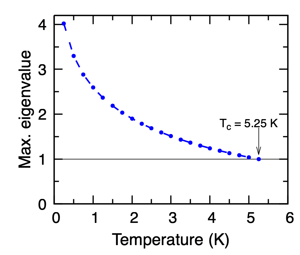
Calculated maximum eigenvalue of the linearised Migdal-Eliashberg kernel as a function of temperature for Pb. \(T_c\) is read off where the curve crosses unity (\(T_c \approx 5.25\) K).
Step 8
The Fermi-surface nesting function \(f_{\rm nest}(\mathbf{q})\) along a high-symmetry path is computed with nest_fn = .true.:
$RUN_EPW -in epw4.in > epw4.out
epw4.in
&INPUTEPW
  prefix      = 'pb',
  amass(1)    = 207.2
  outdir      = './'
  dvscf_dir   = '../phonon/save'

  ep_coupling = .true.
  elph        = .true.
  epwwrite    = .false.
  epwread     = .true.
  etf_mem     = 0
  epw_memdist = .true.

  lifc        = .true.
  asr_typ     = 'crystal'

  wannierize  = .false.
  nbndsub     = 4
  bands_skipped = 'exclude_bands = 1:5'

  fsthick     = 0.2     ! Fermi window thickness [eV]
  degaussw    = 0.05    ! electronic smearing [eV]
  degaussq    = 0.5     ! phonon smearing [meV]

  nest_fn     = .true.  ! Fermi-surface nesting function

  nk1 = 6
  nk2 = 6
  nk3 = 6
  nq1 = 6
  nq2 = 6
  nq3 = 6

  filqf = 'pb_band.kpt'
  nkf1  = 24
  nkf2  = 24
  nkf3  = 24
/
Note. When nest_fn, phonselfen, elecselfen, specfun_el, or specfun_ph is .true., the full (non-reduced) fine \(\mathbf{k}\)-mesh is required, so mp_mesh_k must be .false. (default).
EPW evaluates the Brillouin-zone integral that counts pairs of states separated by \(\mathbf{q}\) and restricted to the Fermi level by two delta functions, for every \(\mathbf{q}\)-point on the path specified by filqf. The values are printed in epw4.out:
===================================================================
Nesting Function in the double delta approx
===================================================================

Fermi Surface thickness =   0.200000 eV
Gaussian Broadening:   0.050 eV, ngauss=   1
DOS =  0.264694 states/spin/eV/Unit Cell at Ef= 10.439436 eV

iq =     1 coord.:   0.00000  0.00000  0.00000 wt:   1.00000
-------------------------------------------------------------------
Nesting function (q)=   0.769610E+03 [Adimensional]
-------------------------------------------------------------------
Extract the \(\mathbf{q}\)-path-resolved nesting function from epw4.out into a two-column file pb.nesting_fn (column 1: q-point index, column 2: nesting value) with a small grep/awk pipeline, then plot:
script_nesting_fn
#!/bin/tcsh
echo "#   iq   Nesting function (q)" > pb.nesting_fn
grep "Nesting function (q)= " epw4.out | awk '{print $4}' | nl >> pb.nesting_fn
plot_nest.gnu
set terminal pngcairo color enhanced font "Times,28" fontscale 1.2 size 1000,850 lw 2
set out "fig6.png"
set border lw 2
set key spacing 1.5
set ytics scale 1.6,0.9
set xtics scale 1.6,0.9
set lmargin screen 0.18
set rmargin screen 0.96
set tmargin screen 0.94
set bmargin screen 0.20
set ylabel "{/=34 f_{nest}(q)}" offset 0.5, 0
set tics font ",32"
set xtics ("{/Symbol G}" 1, "X" 11, "W" 16, "L" 23, "{/Symbol G}" 32, "K" 43)
set ytics 50
set mytics 2
set xrange [1:43]
set yrange [0:175]
set arrow from 11, graph 0 to 11, graph 1 nohead lw 1 dt 2
set arrow from 16, graph 0 to 16, graph 1 nohead lw 1 dt 2
set arrow from 23, graph 0 to 23, graph 1 nohead lw 1 dt 2
set arrow from 32, graph 0 to 32, graph 1 nohead lw 1 dt 2
set key off
plot "pb.nesting_fn" u 1:2 w lp pt 7 ps 1.5 lw 2.5 lc rgb "blue"
reset
Run the helper script and gnuplot:
./script_nesting_fn
gnuplot plot_nest.gnu
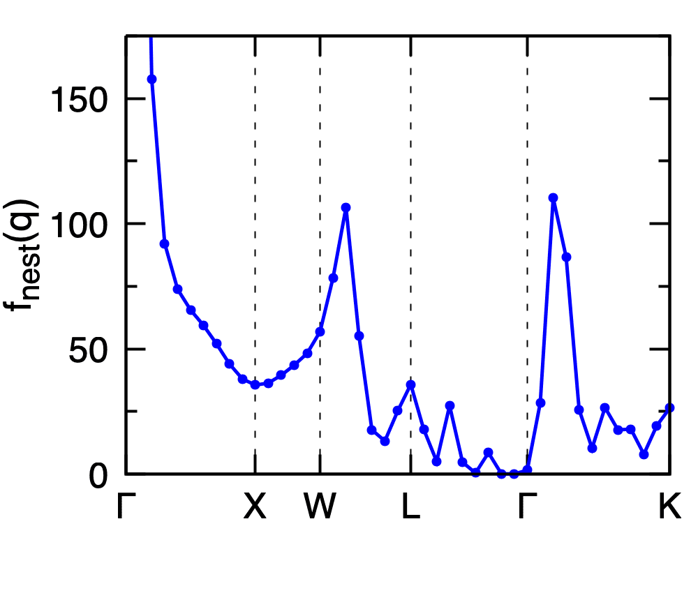
Calculated Fermi-surface nesting function \(f_{\rm nest}(\mathbf{q})\) of Pb along the \(\Gamma\)-X-W-L-\(\Gamma\)-K high-symmetry path.
Exercise 2: Anisotropic superconductivity in MgB2
MgB2 is the standard test case for anisotropic Migdal-Eliashberg calculations because of the two distinct superconducting gaps that open on the \(\sigma\)- and \(\pi\)-derived Fermi sheets. In this exercise we solve the anisotropic gap equations in three flavours and compare them: the Fermi-surface restricted (FSR) approximation, the full-bandwidth (FBW) formulation with uniform Matsubara sampling, and the FBW formulation with sparse-ir Matsubara sampling. The same Wannierised electron-phonon matrix elements are reused across all three runs.
Move to the Exercise 2 directory:
cd exercise2
Step 1
Run SCF on an \(8\times8\times8\) grid and phonons on a \(3\times3\times3\) \(\mathbf{q}\)-grid:
cd phonon
$RUN_PW -in scf.in > scf.out
$RUN_PH -in ph.in  > ph.out
Note. The smearing used here is larger than in published work to keep the run time short. Converge it before production runs.
scf.in
&control
 calculation  = 'scf'
 restart_mode = 'from_scratch'
 prefix       = 'mgb2'
 pseudo_dir   = '../../pseudo/'
 outdir       = './'
/
&system
 ibrav        = 4
 celldm(1)    = 5.8260252227888
 celldm(3)    = 1.1420694129095
 nat          = 3
 ntyp         = 2
 ecutwfc      = 50
 smearing     = 'mp'
 occupations  = 'smearing'
 degauss      = 0.04
/
&electrons
 diagonalization = 'david'
 mixing_mode     = 'plain'
 mixing_beta     = 0.7
 conv_thr        = 1.0d-9
/
ATOMIC_SPECIES
 Mg  24.305  Mg.upf
 B   10.811  B.upf
ATOMIC_POSITIONS crystal
 Mg       0.000000000   0.000000000   0.000000000
 B        0.333333333   0.666666667   0.500000000
 B        0.666666667   0.333333333   0.500000000
K_POINTS automatic
 8 8 8 0 0 0
ph.in
&inputph
  prefix   = 'mgb2'
  outdir   = './'
  fildyn   = 'mgb2.dyn'
  fildvscf = 'dvscf'
  tr2_ph   = 1.0d-14
  ldisp    = .true.
  nq1 = 3
  nq2 = 3
  nq3 = 3
/
The Mg and B norm-conserving pseudopotentials are taken from the PseudoDojo repository (ONCVPSP, scalar-relativistic, PBE).
Step 2
Collect the .dyn, .dvscf, and patterns files into a new save/ directory using the helper script pp.py distributed with EPW:
python3 $QE/../EPW/bin/pp.py
Enter the prefix "mgb2" when prompted.
Compute the inter-atomic force constants and the harmonic phonon dispersion / DOS that will be reused for plotting in Step 4:
$RUN_Q2R    -in q2r.in    > q2r.out
$RUN_MATDYN -in matdyn.in > matdyn.out
$RUN_MATDYN -in phdos.in  > phdos.out
matdyn.in
&INPUT
  asr              = 'crystal',
  flfrc            = 'mgb2.fc',
  flfrq            = 'mgb2.freq',
  dos              = .false.
  q_in_band_form   = .true.,
  q_in_cryst_coord = .true.
/
  8
  0.000 0.000 0.000  50 ! \Gamma
  0.333 0.333 0.000  50 ! K
  0.500 0.000 0.000  50 ! M
  0.000 0.000 0.000  50 ! \Gamma
  0.000 0.000 0.500  50 ! A
  0.333 0.333 0.500  50 ! H
  0.500 0.000 0.500  50 ! L
  0.000 0.000 0.500   1 ! A
Step 3
Run the non-self-consistent calculation on a \(6\times6\times6\) uniform \(\Gamma\)-centred grid and launch the EPW solver for the anisotropic gap in the FSR approximation. The same EPW step Wannierises the bands, writes the mgb2.ephmat/ directory used by the FBW solvers in Step 8 and Step 9, and writes the Eliashberg spectral function mgb2.a2f.
cd ../epw1
$RUN_PW  -in scf.in  > scf.out
$RUN_PW  -in nscf.in > nscf.out
$RUN_EPW -in epw1.in > epw1.out
The 216-point \(6\times6\times6\) \(\mathbf{k}\)-list for nscf.in can be generated with the kmesh.pl utility distributed with Wannier90:
$QE/../wannier90/utility/kmesh.pl 6 6 6
nscf.in
&control
 calculation = 'nscf'
 prefix      = 'mgb2'
 pseudo_dir  = '../../pseudo/'
 outdir      = './'
 verbosity   = 'high'
/
&system
 ibrav       = 4
 celldm(1)   = 5.8260252227888
 celldm(3)   = 1.1420694129095
 nat         = 3
 ntyp        = 2
 ecutwfc     = 50
 smearing    = 'mp'
 occupations = 'smearing'
 degauss     = 0.04
 nbnd        = 16
/
&electrons
 diagonalization = 'david'
 mixing_mode     = 'plain'
 mixing_beta     = 0.7
 conv_thr        = 1.0d-10
/
ATOMIC_SPECIES
 Mg  24.305  Mg.upf
 B   10.811  B.upf
ATOMIC_POSITIONS crystal
 Mg       0.000000000   0.000000000   0.000000000
 B        0.333333333   0.666666667   0.500000000
 B        0.666666667   0.333333333   0.500000000
K_POINTS crystal
 216
 0.00000000  0.00000000  0.00000000  4.629630e-03
 0.00000000  0.00000000  0.16666667  4.629630e-03
 ...
epw1.in
&inputepw
  prefix      = 'mgb2'
  outdir      = './'
  dvscf_dir   = '../phonon/save'

  ep_coupling = .true.
  elph        = .true.
  epwwrite    = .true.
  epwread     = .false.
  etf_mem     = 0
  epw_memdist = .true.

  wannierize    = .true.
  nbndsub       = 5
  num_iter      = 500
  dis_froz_max  = 10.5
  bands_skipped = 'exclude_bands = 1:4'
  proj(1) = 'B:pz'
  proj(2) = 'f=0.5,1.0,0.5:s'
  proj(3) = 'f=0.0,0.5,0.5:s'
  proj(4) = 'f=0.5,0.5,0.5:s'

  iverbosity = 2

  fsthick  = 0.2          ! Fermi window thickness [eV]
  degaussw = 0.05         ! electronic smearing [eV]
  degaussq = 0.5          ! phonon smearing [meV]

  ephwrite   = .true.     ! write mgb2.ephmat/ for the ME solver
  eliashberg = .true.

  laniso = .true.         ! anisotropic Migdal-Eliashberg
  limag  = .true.         ! imaginary-axis equations
  lpade  = .true.         ! Pade continuation
  lacon  = .false.

  nsiter         = 500
  conv_thr_iaxis = 1.0d-4
  wscut          = 0.5    ! Matsubara cutoff [eV]
  muc            = 0.1    ! effective Coulomb parameter

  nstemp = 9
  temps  = 5 45           ! evenly spaced nstemp points

  nk1 = 6
  nk2 = 6
  nk3 = 6
  nq1 = 3
  nq2 = 3
  nq3 = 3

  mp_mesh_k = .true.
  nkf1 = 40
  nkf2 = 40
  nkf3 = 40
  nqf1 = 20
  nqf2 = 20
  nqf3 = 20
/
EPW interpolates the electron-phonon matrix elements onto the dense \(40\times40\times40\) \(\mathbf{k}\)-grid and \(20\times20\times20\) \(\mathbf{q}\)-grid, restricts to \(\mathbf{q}\)-points within the Fermi window, writes the mgb2.ephmat/ directory, and then solves the anisotropic FSR Migdal-Eliashberg equations at the temperatures listed in temps. Pade continuation to the real axis follows immediately; the iterative continuation (lacon) is disabled here because it is expensive in the anisotropic case.
Expected output (truncated):
===================================================================
Solve anisotropic Eliashberg equations
===================================================================

             Fermi level (eV) =     9.2339726551E+00
DOS(states/spin/eV/Unit Cell) =     3.9470128030E-01
       Electron smearing (eV) =     5.0000000000E-02
            Fermi window (eV) =     2.0000000000E-01
Nr irreducible k-points within the Fermi shell =       448 out of      3234

      2 bands within the Fermi window
Max nr of q-points =      1098

Electron-phonon coupling strength =    0.5729486

Estimated Tc using McMillan expression =  14.1859 K for muc =   0.1000
Estimated Tc using Allen-Dynes modified McMillan expression =  14.5549 K
Estimated Tc using SISSO machine learning model =  14.0296 K
Estimated w_log =  61.7402 meV
Estimated BCS superconducting gap using McMillan Tc =   2.1515 meV

Actual number of frequency points (     1) =    185 for uniform sampling

temp(  1) =      5.00000 K

Solve anisotropic Eliashberg equations on imaginary-axis

Total number of frequency points nsiw(     1) =    185
   iter      ethr          znormi      deltai [meV]
     1   3.052298E+00   1.559224E+00   2.384930E+00
     ...
     69   5.044619E-05   1.553563E+00   3.955953E+00
Convergence was reached in nsiter =     69
EPW writes one set of files per temperature; XX denotes the temperature tag (e.g. 005.00 for \(T = 5\) K):
mgb2.lambda_pairs– distribution of the anisotropic coupling \(\lambda_{n\mathbf{k},\,m\mathbf{k}+\mathbf{q}}(0)\).mgb2.lambda_k_pairs– band- and wave-vector-resolved coupling \(\lambda_{n\mathbf{k}}(0)\) on the Fermi surface.mgb2.lambda.frmsf– Fermi-surface representation of \(\lambda_{n\mathbf{k}}(0)\) for Fermisurfer.mgb2.a2f– isotropic \(\alpha^2 F(\omega)\) and cumulative \(\lambda(\omega)\) for several phonon smearing values.mgb2.imag_aniso_XX– Matsubara frequency, Kohn-Sham eigenvalue relative to \(E_F\), renormalisation \(Z_{n\mathbf{k}}\), gap \(\Delta_{n\mathbf{k}}\) (eV).mgb2.pade_aniso_XX– real-axis frequency and the real/imaginary parts of \(Z\) and \(\Delta\) (eV) from Pade continuation.mgb2.imag_aniso_gap0_XX– distribution of leading-edge gap values used to plot \(\Delta_{n\mathbf{k}}(T)\).mgb2.qdos_XX– superconducting quasiparticle density of states relative to the normal-state DOS at \(E_F\).
Note. Before plotting mgb2.a2f with gnuplot, comment out (with #) the first header line and the last seven lines that give smearing metadata.
Step 4
Combine the harmonic phonon dispersion and DOS produced in Step 2 with the spectral function mgb2.a2f written in Step 3 using the following gnuplot script:
plot_phbands.gnu
set terminal pngcairo color enhanced font "Times,30" fontscale 1.0 size 1400,900 lw 2
set out "mgb2_fig1.png"
set multiplot
set border lw 1.75

ymin = 0
ymax = 100.5
set yrange [ymin:ymax]
set ytics 20
set mytics 2
set ytics scale 1.2,0.8
set xtics scale 1.2,0.8

# Panel 1: Phonon dispersion (left)
set lmargin at screen 0.10
set rmargin at screen 0.57
set bmargin at screen 0.18
set tmargin at screen 0.95
set ylabel "{/Symbol w} (meV)" offset 1,0
set xtics ("{/Symbol G}" 0, "K" 0.6660, "M" 0.9990, "{/Symbol G}" 1.5763, "A" 2.0142, "H" 2.6802, "L" 3.0131, "A" 3.5905) nomirror
set xrange [0:3.5905]
set arrow 1 from 0.6660, graph 0 to 0.6660, graph 1 nohead lw 1.0 dt 2
set arrow 2 from 0.9990, graph 0 to 0.9990, graph 1 nohead lw 1.0 dt 2
set arrow 3 from 1.5763, graph 0 to 1.5763, graph 1 nohead lw 1.0 dt 2
set arrow 4 from 2.0142, graph 0 to 2.0142, graph 1 nohead lw 1.0 dt 2
set arrow 5 from 2.6802, graph 0 to 2.6802, graph 1 nohead lw 1.0 dt 2
set arrow 6 from 3.0131, graph 0 to 3.0131, graph 1 nohead lw 1.0 dt 2
unset key
plot "../phonon/mgb2.freq.gp" u 1:($2/8.06554) w l lw 2 lt -1, \
     "../phonon/mgb2.freq.gp" u 1:($3/8.06554) w l lw 2 lt -1, \
     "../phonon/mgb2.freq.gp" u 1:($4/8.06554) w l lw 2 lt -1, \
     "../phonon/mgb2.freq.gp" u 1:($5/8.06554) w l lw 2 lt -1, \
     "../phonon/mgb2.freq.gp" u 1:($6/8.06554) w l lw 2 lt -1, \
     "../phonon/mgb2.freq.gp" u 1:($7/8.06554) w l lw 2 lt -1, \
     "../phonon/mgb2.freq.gp" u 1:($8/8.06554) w l lw 2 lt -1, \
     "../phonon/mgb2.freq.gp" u 1:($9/8.06554) w l lw 2 lt -1, \
     "../phonon/mgb2.freq.gp" u 1:($10/8.06554) w l lw 2 lt -1

# Panel 2: Phonon DOS (middle)
set lmargin at screen 0.59
set rmargin at screen 0.77
set bmargin at screen 0.18
set tmargin at screen 0.95
unset arrow
unset ylabel
set format y ""
set xlabel "PhDOS\n(states/meV)"
set xrange [0:0.7]
unset xtics
set xtics 0.3 nomirror
set xtics scale 1.2,0.8
set mxtics 2
unset key
plot "../phonon/mgb2.phdos" u ($2*8.06554):($1/8.06554) w l lw 2.5 lt -1

# Panel 3: a2f and lambda (right)
set lmargin at screen 0.79
set rmargin at screen 0.97
set bmargin at screen 0.18
set tmargin at screen 0.95
set format y ""
set ytics nomirror
set xlabel "{/Symbol a}^2F({/Symbol w}), {/Symbol l}({/Symbol w})"
set xrange [0:1.0]
unset xtics
set xtics 0.5 nomirror
set xtics scale 1.2,0.8
set mxtics 2
set key at graph 0.95, 0.05 bottom right reverse Left samplen 2 spacing 1.3 nobox
plot "mgb2.a2f" u 2:1 w l lw 2.5 lt -1 title "{/Symbol a}^2F", \
     "mgb2.a2f" u 3:1 w l lw 2.5 lt 1 lc rgb "red" dt (6,3) title "{/Symbol l}"

unset multiplot
unset out
Run the script with gnuplot:
gnuplot plot_phbands.gnu
Calculated phonon dispersion (left), phonon density of states (middle), and isotropic Eliashberg spectral function \(\alpha^2 F(\omega)\) with the cumulative electron-phonon coupling \(\lambda(\omega)\) (right) of MgB2. The high-frequency \(E_{2g}\) boron-stretching modes around 60-80 meV give the dominant contribution to \(\lambda\).
Plot the anisotropy of the coupling on the Fermi surface with the following gnuplot script (the third panel embeds an external Fermisurfer screenshot mgb2_lambda.png):
plot_lambda_aniso.gnu
set terminal pngcairo color enhanced font "Times,30" fontscale 1.0 size 1500,480 lw 2
set out "mgb2_fig2.png"
set multiplot
set border lw 1.75

set ytics scale 1.2,0.8
set xtics scale 1.2,0.8

# Panel 1: lambda_{nk,mk+q} distribution
set lmargin at screen 0.13
set rmargin at screen 0.36
set tmargin at screen 0.92
set bmargin at screen 0.24
set xlabel "{/Symbol l}_{nk,mk+q}" offset 0,0.5
set ylabel "{/Symbol r}({/Symbol l}_{nk,mk+q})" offset 0.8,0
set xtics 1 nomirror
set mxtics 2
set ytics 0.5 nomirror
set mytics 2
set xrange [0:3]
set yrange [0:1.2]
unset key
plot "mgb2.lambda_pairs" w l lw 2.5 lt -1

# Panel 2: lambda_{nk} distribution
set lmargin at screen 0.46
set rmargin at screen 0.68
set tmargin at screen 0.92
set bmargin at screen 0.24
set xlabel "{/Symbol l}_{nk}" offset 0,0.5
set ylabel "{/Symbol r}({/Symbol l}_{nk})" offset 1.4,0
set xtics 0.5 nomirror
set mxtics 2
set ytics 0.5 nomirror
set mytics 2
set xrange [0:1.2]
set yrange [0:1.2]
unset key
plot "mgb2.lambda_k_pairs" w l lw 2.5 lt -1

# Panel 3: lambda image (Fermisurfer screenshot saved as mgb2_lambda.png)
set lmargin at screen 0.70
set rmargin at screen 0.90
set tmargin at screen 0.92
set bmargin at screen 0.24
unset xlabel
unset ylabel
unset xtics
unset ytics
unset border
unset key
set xrange [*:*]
set yrange [*:*]
set autoscale fix
plot "mgb2_lambda.png" binary filetype=png with rgbalpha notitle

unset multiplot
unset out
Run the script with gnuplot:
gnuplot plot_lambda_aniso.gnu
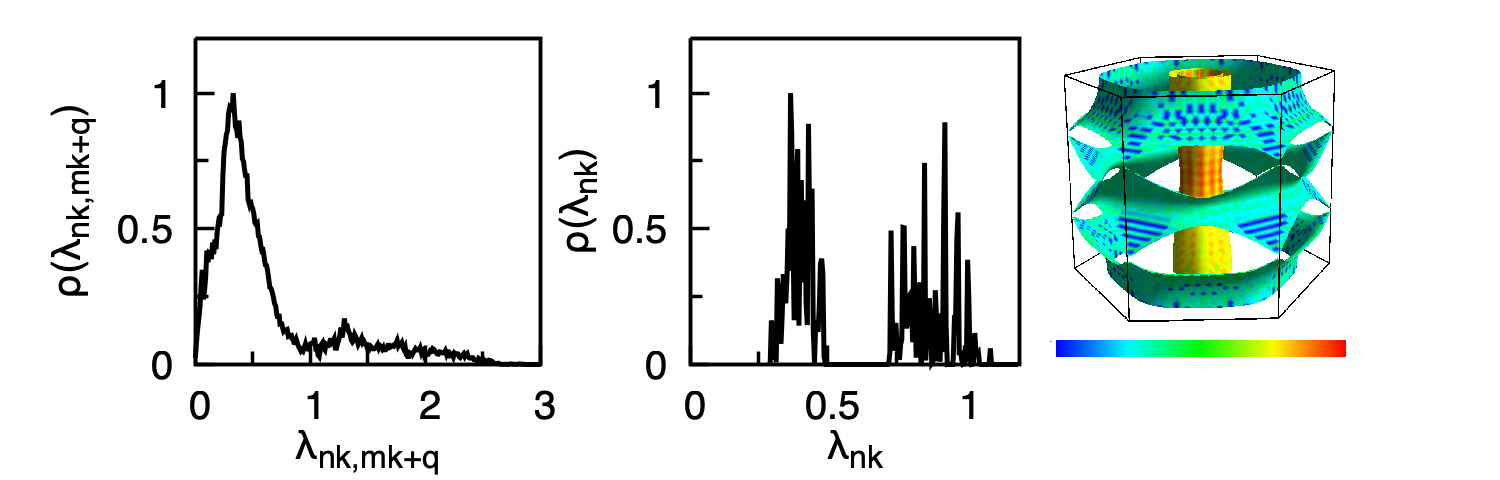
Left: distribution of the pair coupling \(\lambda_{n\mathbf{k},\,m\mathbf{k}+\mathbf{q}}(0)\) from mgb2.lambda_pairs. Middle: distribution of the state-resolved coupling \(\lambda_{n\mathbf{k}}(0)\) on the Fermi surface from mgb2.lambda_k_pairs. Right: anisotropic electron-phonon coupling \(\lambda_{n\mathbf{k}}(0)\) plotted on the Fermi surface with Fermisurfer from mgb2.lambda.frmsf; the two \(\sigma\)-cylinders and the \(\pi\)-honeycomb sheets are clearly resolved.
Step 5
Plot the anisotropic gap on the imaginary and real axes at \(T = 5\) K with the following gnuplot script:
plot_gap_aniso_conv.gnu
set terminal pngcairo color enhanced font "Times,30" fontscale 1.0 size 1400,600 lw 2
set out "mgb2_fig3.png"
set multiplot
set border lw 1.75

set ytics scale 1.2,0.8
set xtics scale 1.2,0.8

# Panel 1: Delta_{nk} on imaginary axis
set lmargin at screen 0.09
set rmargin at screen 0.48
set tmargin at screen 0.92
set bmargin at screen 0.22
set ylabel "{/Symbol D}_{nk} (meV)" offset 0.8,0
set xlabel "i{/Symbol w} (meV)" offset 0,0.5
set xtics 40 nomirror
set mxtics 2
set ytics 3 nomirror
set mytics 3
set xrange [0:180]
set yrange [-1:9]
unset key
plot "mgb2.imag_aniso_005.00" u ($1*1000):($4*1000) w p pt 7 ps 0.4 lc rgb "black" notitle

# Panel 2: Re Delta - Pade approximation
set lmargin at screen 0.58
set rmargin at screen 0.97
set tmargin at screen 0.92
set bmargin at screen 0.22
set ylabel "{/Symbol D}_{nk} (meV)" offset 0.9,0
set xlabel "{/Symbol w} (meV)" offset 0,0.5
set xtics 40 nomirror
set mxtics 2
set ytics 20 nomirror
set mytics 2
set xrange [0:180]
set yrange [-20:40]
set label 1 "Re{/Symbol D} - Pade approx." font "Times,24" at graph 0.45, 0.92
unset key
plot "mgb2.pade_aniso_005.00" u ($1*1000):($5*1000) w p pt 7 ps 0.35 lc rgb "black" notitle

unset multiplot
unset out
Run the script with gnuplot:
gnuplot plot_gap_aniso_conv.gnu
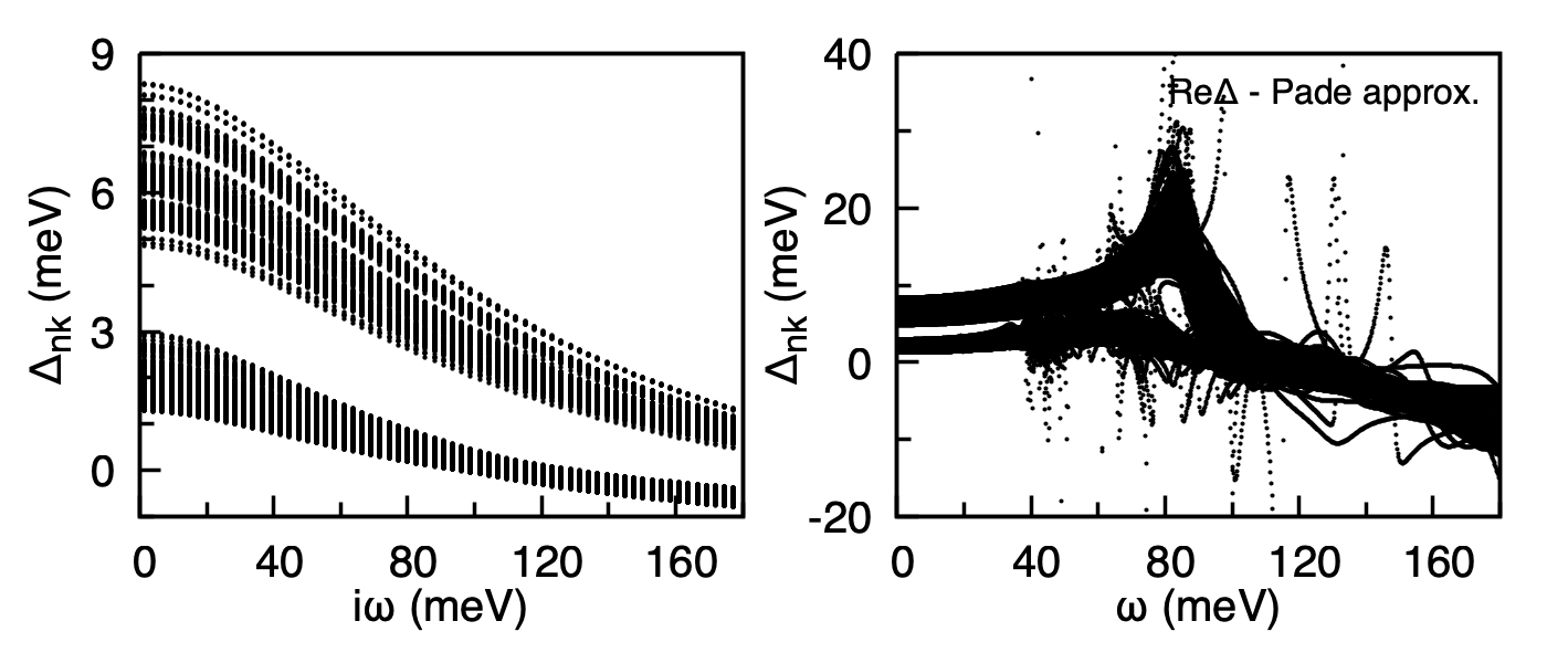
Anisotropic superconducting gap of MgB2 at \(T = 5\) K. Left: imaginary-axis \(\Delta_{n\mathbf{k}}(i\omega_n)\) from mgb2.imag_aniso_005.00. Right: real part of the real-axis gap \({\rm Re}\,\Delta_{n\mathbf{k}}(\omega)\) from mgb2.pade_aniso_005.00 obtained by Pade continuation. The two-gap structure (small \(\pi\)-gap, large \(\sigma\)-gap) is clearly resolved.
Step 6
Collect the leading-edge gap distribution at every temperature from the mgb2.imag_aniso_gap0_XX files and plot the temperature dependence in the FSR approximation with the following gnuplot script:
plot_gap_fsr.gnu
set terminal pngcairo color enhanced font "Times,30" fontscale 1.0 size 800,700 lw 2
set out "mgb2_fig4.png"
set border lw 1.75

set ytics scale 1.2,0.8
set xtics scale 1.2,0.8

set lmargin at screen 0.18
set rmargin at screen 0.95
set tmargin at screen 0.92
set bmargin at screen 0.18

set ylabel "{/Symbol D}_{nk} (meV)" offset 0.8,0
set xlabel "Temperature (K)" offset 0,0.3
set xtics 10 nomirror
set mxtics 2
set ytics 4 nomirror
set mytics 2
set xrange [0:52]
set yrange [0:8.25]
unset key

scale = 3E-3
set label 1 "FSR ({/Symbol m}_c^*=0.1)" font "Times,22" at graph 0.65, 0.93
set style fill transparent solid 0.2

plot \
  for [temp in "5 10 15 20 25 30 35 40"] gprintf('./mgb2.imag_aniso_gap0_%06.2f', temp) u (($3)+scale*($5)):($2) with filledc above x1=temp lc rgb "blue" dt 1 lw 0 notitle, \
  for [temp in "5 10 15 20 25 30 35 40"] gprintf('./mgb2.imag_aniso_gap0_%06.2f', temp) u (($3)+scale*($5)):($2) w l lc rgb "blue" dt 1 lw 1 notitle

unset out
Run the script with gnuplot:
gnuplot plot_gap_fsr.gnu
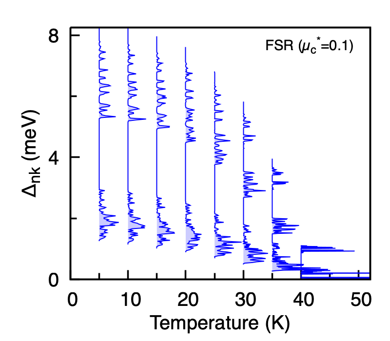
Calculated anisotropic superconducting gap of MgB2 on the Fermi surface as a function of temperature, from the FSR Migdal-Eliashberg solver with \(\mu_c^{*} = 0.1\). The two distinct gaps merge and close at \(T_c\).
Step 7
The superconducting quasiparticle DOS, \(N_s(\omega)\), normalised to the normal-state DOS at \(E_F\), \(N_F\), is read from mgb2.qdos_XX. The normalisation factor \(N_F\) is the value of DOS(states/spin/eV/Unit Cell) printed in epw1.out. Update the NF constant inside the script with that value, then plot at \(T = 5\) K:
plot_qdos.gnu
set terminal pngcairo color enhanced font "Times,30" fontscale 1.0 size 800,700 lw 2
set out "mgb2_fig5.png"
set border lw 1.75

set ytics scale 1.2,0.8
set xtics scale 1.2,0.8

set lmargin at screen 0.18
set rmargin at screen 0.95
set tmargin at screen 0.92
set bmargin at screen 0.18

set ylabel "N_s({/Symbol w})/N_F" offset 1.2,0
set xlabel "{/Symbol w} (meV)" offset 0,0.4
set xtics 5 nomirror
set mxtics 2
set ytics 0.5 nomirror
set mytics 2
set xrange [0:15]
set yrange [0:2]
unset key

NF = 0.340839995110793           # normal-state DOS at E_F (from epw1.out)
plot "mgb2.qdos_005.00" u ($1*1000):($2/NF) w l lw 2.5 lt -1 notitle

unset out
Run the script with gnuplot:
gnuplot plot_qdos.gnu
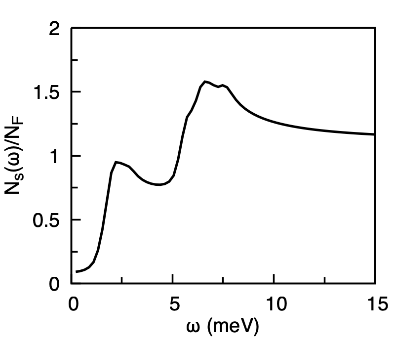
Normalised superconducting quasiparticle density of states \(N_s(\omega)/N_F\) of MgB2 at \(T = 5\) K. The two coherence peaks correspond to the \(\pi\) and \(\sigma\) gaps.
Step 8
The FSR approximation linearises the Migdal-Eliashberg equations around \(E_F\). The full-bandwidth (FBW) formulation keeps the explicit dependence on the Kohn-Sham eigenvalue and self-consistently updates the chemical potential through the energy shift \(\chi_{n\mathbf{k}}(i\omega_n)\); this is important when the DOS varies appreciably across the Fermi window or when the gap-to-bandwidth ratio is not small. We start with uniform Matsubara sampling.
Reuse the Wannier files written by epw1.in and run a second EPW job in the epw2 directory:
cd ../epw2
ln -s ../epw1/*.fmt    .
ln -s ../epw1/mgb2.ephmat .
ln -s ../epw1/mgb2.a2f    .
ln -s ../epw1/mgb2.dos    .
ln -s ../epw1/mgb2.ukk    .
$RUN_EPW -in epw2.in > epw2.out
epw2.in
&inputepw
  prefix      = 'mgb2'
  outdir      = './'
  dvscf_dir   = '../phonon/save'

  ep_coupling = .false.
  elph        = .false.
  epwwrite    = .false.
  epwread     = .true.
  etf_mem     = 0

  wannierize  = .false.
  nbndsub     = 5

  iverbosity  = 2

  fsthick     = 0.2       ! Fermi window thickness [eV]
  degaussw    = 0.05      ! electronic smearing [eV]
  degaussq    = 0.5       ! phonon smearing [meV]

  ephwrite    = .false.
  eliashberg  = .true.

  laniso = .true.         ! anisotropic Migdal-Eliashberg
  fbw    = .true.         ! full-bandwidth formulation
  limag  = .true.
  lpade  = .true.
  lacon  = .false.

  nsiter         = 500
  conv_thr_iaxis = 1.0d-4
  wscut          = 0.5    ! eV
  muc            = 0.1

  nstemp = 10
  temps  = 5 50

  nk1 = 6
  nk2 = 6
  nk3 = 6
  nq1 = 3
  nq2 = 3
  nq3 = 3

  mp_mesh_k = .true.
  nkf1 = 40
  nkf2 = 40
  nkf3 = 40
  nqf1 = 20
  nqf2 = 20
  nqf3 = 20
/
Step 9
In the conventional (uniform) Matsubara representation the number of frequency points needed to resolve the gap and self-energy at low temperature grows \(\propto 1/T\). The
sparse intermediate-representation (sparse-ir) of H. Shinaoka et al., Phys. Rev. B 96, 035147 (2017) replaces the uniform grid with a small set of basis functions and a non-uniform sampling mesh that captures the same information with far fewer points. In EPW the sparse-ir sampling is activated with gridsamp = 2; the basis functions and sampling points are read from a pre-computed object file pointed at by filirobj. With sparse-ir sampling the number of Matsubara points required for a given numerical accuracy is typically much smaller than with uniform sampling, so runs that would be infeasible on a dense Matsubara grid become tractable. EPW cannot generate the sparse-ir object file itself; produce it beforehand with the Python sparse-ir package (see sparse-ir-fortran). The filename pattern ir_nlambda<N>_ndigit<M>.dat encodes \(\Lambda = 10^N\) (maximum Matsubara frequency) and \(\epsilon_{\rm IR} = 10^{-M}\) (basis accuracy); larger \(N\) or \(M\) yield more sampling points.
Run the FBW solver again, this time with sparse-ir Matsubara sampling, in the epw3 directory. The same mgb2.ephmat/ and *.fmt files written in Step 3 are reused:
cd ../epw3
ln -s ../epw1/*.fmt       .
ln -s ../epw1/mgb2.ephmat .
ln -s ../epw1/mgb2.a2f    .
ln -s ../epw1/mgb2.dos    .
ln -s ../epw1/mgb2.ukk    .
$RUN_EPW -in epw3.in > epw3.out
epw3.in
&inputepw
  prefix      = 'mgb2'
  outdir      = './'
  dvscf_dir   = '../phonon/save'

  ep_coupling = .false.
  elph        = .false.
  epwwrite    = .false.
  epwread     = .true.
  etf_mem     = 0

  wannierize  = .false.
  nbndsub     = 5

  iverbosity  = 2

  fsthick     = 0.2       ! Fermi window thickness [eV]
  degaussw    = 0.05      ! electronic smearing [eV]
  degaussq    = 0.5       ! phonon smearing [meV]

  ephwrite    = .false.
  eliashberg  = .true.

  laniso   = .true.
  fbw      = .true.
  limag    = .true.
  lpade    = .false.
  lacon    = .false.
  gridsamp = 2            ! sparse-ir Matsubara sampling
  filirobj = '../../sparse-ir/ir_nlambda6_ndigit8.dat'
  broyden_beta = -0.7     ! linear mixing (negative = linear)

  nsiter         = 500
  conv_thr_iaxis = 1.0d-4
  wscut          = 0.5    ! eV
  muc            = 0.1

  nstemp = 10
  temps  = 5 50

  nk1 = 6
  nk2 = 6
  nk3 = 6
  nq1 = 3
  nq2 = 3
  nq3 = 3

  mp_mesh_k = .true.
  nkf1 = 40
  nkf2 = 40
  nkf3 = 40
  nqf1 = 20
  nqf2 = 20
  nqf3 = 20
/
Note 1. With gridsamp = 2, the Matsubara frequencies are read from the sparse-ir object file, so wscut is used only to set the upper limit of the real frequency axis during analytic continuation.
Note 2. From EPW v5.8 onwards, ephmatXX files can be reread with a different number of MPI pools than used when they were written, which makes the ln -s reuse pattern above safe.
Note 3. For anisotropic FBW runs, linear mixing (broyden_beta < 0) often converges more reliably than Broyden mixing.
During the run EPW prints the actual number of Matsubara sampling points, which should be much smaller than the uniform-grid number at the same cutoff:
===================================================================
Solve full-bandwidth anisotropic Eliashberg equations
===================================================================

             Fermi level (eV) =     9.2339726551E+00
DOS(states/spin/eV/Unit Cell) =     3.9470128030E-01

Start reading ir object file
Finish reading ir object file

Actual number of frequency points (     1) =     48 for sparse-ir sampling

temp(  1) =      5.00000 K

Solve full-bandwidth anisotropic Eliashberg equations on imaginary-axis

Total number of frequency points nsiw(     1) =     48
Parameters for IR basis: Lambda = 1.00E+06, eps_IR = 1.00E-08
Maximum frequency =      3296.9453 eV
linear mixing factor =      0.70000

   iter      ethr          znormi      deltai [meV]   shifti [meV]       mu [eV]
     1   1.832096E+00   1.410063E+00   2.662866E+00  -1.661467E+00   9.233973E+00
     ...
     27   8.572808E-05   1.372192E+00   4.744748E+00  -7.239758E-01   9.233973E+00
Convergence was reached in nsiter =     27
For comparison, the uniform sampling at the same wscut (epw2.in) requires on the order of 185 Matsubara points at \(T = 5\) K, while sparse-ir sampling needs only 48.
Step 10
Combine the leading-edge gap distributions mgb2.imag_aniso_gap0_XX from the three EPW runs to compare the FSR approximation, FBW with uniform sampling, and FBW with sparse-ir sampling on a single plot. Run the script from the epw1 directory; it pulls the FBW data from ../epw2 and ../epw3.
plot_gap_fbw.gnu
set terminal pngcairo color enhanced font "Times,30" fontscale 1.0 size 800,700 lw 2
set out "mgb2_fig6.png"
set border lw 1.75

set ytics scale 1.2,0.8
set xtics scale 1.2,0.8

set lmargin at screen 0.18
set rmargin at screen 0.95
set tmargin at screen 0.92
set bmargin at screen 0.18

set ylabel "{/Symbol D}_{nk} (meV)" offset 0.8,0
set xlabel "Temperature (K)" offset 0,0.3
set xtics 10 nomirror
set mxtics 2
set ytics 4 nomirror
set mytics 2
set xrange [0:52]
set yrange [0:10]

set key at graph 0.97, 0.97 right top samplen 2 spacing 1.2 font "Times,22" width 1

scale = 3E-3
set label 1 "{/Symbol m}_c^*=0.1" font "Times,22" at graph 0.03, 0.93
set style fill transparent solid 0.2

plot \
  for [temp in "5 10 15 20 25 30 35 40"] gprintf('./mgb2.imag_aniso_gap0_%06.2f',       temp) u (($3)+scale*($5)):($2) with filledc above x1=temp lc rgb "blue"      dt 1 lw 0 notitle, \
  for [temp in "5 10 15 20 25 30 35 40"] gprintf('./mgb2.imag_aniso_gap0_%06.2f',       temp) u (($3)+scale*($5)):($2) w l lc rgb "blue"      dt 1 lw 1 notitle, \
  for [temp in "5 10 15 20 25 30 35 40"] gprintf('../epw2/mgb2.imag_aniso_gap0_%06.2f', temp) u (($3)+scale*($5)):($2) with filledc above x1=temp lc rgb "red"       dt 1 lw 0 notitle, \
  for [temp in "5 10 15 20 25 30 35 40"] gprintf('../epw2/mgb2.imag_aniso_gap0_%06.2f', temp) u (($3)+scale*($5)):($2) w l lc rgb "red"       dt 1 lw 1 notitle, \
  for [temp in "5 10 15 20 25 30 35 40"] gprintf('../epw3/mgb2.imag_aniso_gap0_%06.2f', temp) u (($3)+scale*($5)):($2) with filledc above x1=temp lc rgb "#80006400" dt 1 lw 0 notitle, \
  for [temp in "5 10 15 20 25 30 35 40"] gprintf('../epw3/mgb2.imag_aniso_gap0_%06.2f', temp) u (($3)+scale*($5)):($2) w l lc rgb "#80006400" dt 1 lw 1 notitle, \
  NaN w l lc rgb "blue"      lw 2.5 title "FSR", \
  NaN w l lc rgb "red"       lw 2.5 title "FBW", \
  NaN w l lc rgb "#80006400" lw 2.5 title "FBW (sparse-IR)"

unset out
Run the script with gnuplot:
cd ../epw1
gnuplot plot_gap_fbw.gnu
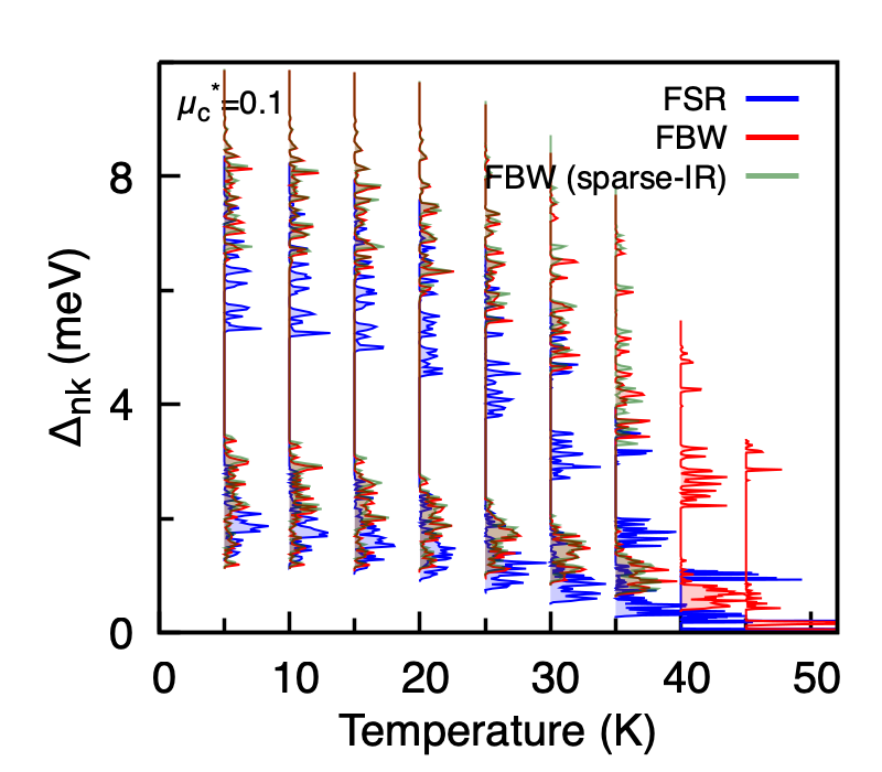
Calculated anisotropic superconducting gap of MgB2 on the Fermi surface as a function of temperature, comparing the FSR solver (blue), the FBW solver with uniform Matsubara sampling (red), and the FBW solver with sparse-ir Matsubara sampling (green). The FBW results are nearly indistinguishable between uniform and sparse-ir sampling, while the FBW gap closes at a higher \(T_c\) than the FSR gap – the expected effect of restoring the energy dependence of the self-energies and the chemical-potential update.
Appendix: Restart options
EPW supports three restart modes that cover the usual iteration patterns of a superconductivity workflow.
Restart from the Wannier-representation matrix elements (
prefix.epmatwp,epwdata.fmt). Useful when changing any ofnkf1-3,nqf1-3,fsthick, ordegaussw. Deleteprefix.ephmat,restart.fmt,selecq.fmt, andprefix.a2fbefore restarting. Required files:prefix.epmatwp,prefix.ukk,crystal.fmt,epwdata.fmt, andvmedata.fmt(ordmedata.fmt).ep_coupling = .true. elph = .true. epwwrite = .false. epwread = .true. wannierize = .false. ephwrite = .true.
The number of MPI pools may differ from the original run.
Restart an interrupted q-loop during
ephmatXXwriting. Required files:prefix.epmatwp,prefix.ukk,crystal.fmt,epwdata.fmt,vmedata.fmt(ordmedata.fmt),restart.fmt, andselecq.fmt(selecq.fmtonly ifselecqread = .true.; otherwise it is regenerated).ep_coupling = .true. elph = .true. epwwrite = .false. epwread = .true. wannierize = .false. ephwrite = .true.
The number of MPI pools must match the original run.
Restart from the saved
ephmatXXfiles. Required files: theprefix.ephmat/directory (withegnv,freq,ikmap, and theephmatXXfiles),prefix.dos,selecq.fmt, andcrystal.fmt.ep_coupling = .false. elph = .false. wannierize = .false. ephwrite = .false.
From EPW v5.8 onwards,
ephmatXXfiles may be read back with a different number of MPI pools.