Phonon-assisted optical processes

Amanda Wang 07/08/2026
Sabyasachi Tiwari (2024), Xiao Wang (2022, 2024)

Note

Hands-on based on Quantum ESPRESSO v7.6 and EPW v6.1.

Introduction

In this tutorial, we will show how to compute the optical absorption spectra of Si and GaAs. The examples cover phonon-assisted optical absorption using second-order perturbation theory, free-carrier absorption, and direct and phonon-assisted absorption using quasi-degenerate perturbation theory.

The following job submission script, run.sh, has been prepared:

run.sh

#!/bin/bash
#SBATCH -J job.ph # Job name
#SBATCH -N 1 # Total # of nodes
#SBATCH --ntasks-per-node 56
#SBATCH -t 00:15:00 # Run time (hh:mm:ss)
#SBATCH -A DMR23048
#SBATCH -p normal
#SBATCH --reservation=MATCSSI_Norm_June18

# Launch MPI code...
module load hdf5/1.10.4
export PATHQE=/work2/05193/sabyadk/shared/EPW_6.1s/q-e

ibrun $PATHQE/bin/pw.x < scf.in | tee scf.out
ibrun $PATHQE/bin/ph.x < ph.in | tee ph.out

To run each step below, copy this script into the working folder, replace the ibrun commands with the command provided in the corresponding step, and submit the job using:

$ sbatch run.sh

To run the post-processing commands on the login node, we need to define the path to the post-processing scripts. Run the following commands to define the shortcut to the scripts:

$ module load hdf5/1.10.4
$ export PATHQE=/work2/05193/sabyadk/shared/EPW_6.1s/q-e

For descriptions of all EPW input flags, please follow the link:

https://docs.epw-code.org/Inputs/Inputs.html

Exercise 1: Optical absorption in Si

1.1 Preliminary calculations with Quantum Espresso

In this example we are going to calculate the optical absorption spectra of Si using two approaches: second-order perturbation theory to calculate phonon-assisted optical absorption and quasi-degenerate perturbation theory to calculate both direct and phonon-assisted optical absorption.

First download the exercise files, then go into the exercise1/ directory.

$ cd $SCRATCH
$ wget --content-disposition \
  "https://drive.google.com/uc?export=download&id=1G0k5G7S6u31PSPuXG1R6l9nC-wRmEIKN"
$ tar -xvf Thu.6.Wang.tar
$ cd Thu.6.Wang/exercise1/

Action. Make a self-consistent calculation for Si.

scf.in

&control
    calculation     = 'scf'
    prefix          = 'si'
    restart_mode    = 'from_scratch'
    pseudo_dir      = './'
    outdir          = './'
 /
 &system
    ibrav           = 2
    celldm(1)       = 10.262
    nat             = 2
    ntyp            = 1
    ecutwfc         = 20
 /
 &electrons
    diagonalization = 'david'
    mixing_beta     = 0.7
    conv_thr        = 1.0d-13
 /
ATOMIC_SPECIES
  Si  28.0855  Si_r.upf
ATOMIC_POSITIONS alat
  Si   0.00  0.00  0.00
  Si   0.25  0.25  0.25
K_POINTS automatic
12 12 12 0 0 0

Note: The k-point grid needs to be fairly dense in order to get converged dielectric function and Born effective charge during the following phonon calculation.

$ ibrun -np 8 $PATHQE/bin/pw.x -npool 8 < scf.in > scf.out

Action. Compute the vibrational properties of Si on a coarse \(3\times3\times3\) \(\mathbf{q}\)-point grid.

ph.in

&inputph
  prefix   = 'si',
  epsil    = .false.,
  fildyn   = 'si.dyn',
  ldisp    = .true.
  fildvscf = 'dvscf'
  nq1=3,
  nq2=3,
  nq3=3,
  tr2_ph   =  1.0d-14,
 /

$ ibrun -np 56 $PATHQE/bin/ph.x -npool 28 < ph.in > ph.out

During the run, notice the IBZ q-point grid. You can look at the output file or simply use the following command:

grep -6 Dynamical ph.out | tail -7

Dynamical matrices for ( 3, 3, 3)  uniform grid of q-points
(   4 q-points):
  N         xq(1)         xq(2)         xq(3)
  1   0.000000000   0.000000000   0.000000000
  2  -0.333333333   0.333333333  -0.333333333
  3   0.000000000   0.666666667   0.000000000
  4   0.666666667  -0.000000000   0.666666667

We also obtain the dielectric function and Born effective charge tensor. You can look at the output file or simply use the following command

grep -15 'Dielectric constant in' ph.out | tail -17

    Dielectric constant in cartesian axis

    (      12.982914367       0.000000000       0.000000000 )
    (       0.000000000      12.982914367      -0.000000000 )
    (      -0.000000000      -0.000000000      12.982914367 )

    Effective charges (d Force / dE) in cartesian axis

     atom      1   Si
Ex  (       -0.00778        0.00000        0.00000 )
Ey  (        0.00000       -0.00778       -0.00000 )
Ez  (        0.00000       -0.00000       -0.00778 )
     atom      2   Si
Ex  (       -0.00778       -0.00000       -0.00000 )
Ey  (       -0.00000       -0.00778       -0.00000 )
Ez  (        0.00000       -0.00000       -0.00778 )

The experimental dielectric constant of silicon is about 11.9 so that we overestimate it a bit. A smaller value can be obtained with larger \(\mathbf{k}\)-point grids but DFT will always overestimate experiment. Since Si is a nonpolar material, the Born effective charges should be 0. Indeed, one can see that we are close to zero. In a converged calculation you may want to get an even smaller value.

Action. Run the python post-processing to create the save folder (No job submission needed, can be run simply on the login node.)

$  python3 $PATHQE/EPW/bin/pp.py

The script will ask you to enter the prefix used for the calculation. In this case enter “si”. The script will create a new folder called “save” that contains the dvscf potential files, pattern files, and dynamical matrices on the IBZ.

1.2 Interpolation of the electron-phonon matrix elements with EPW

Action. Do a non-self-consistent calculation on a homogeneous \(6\times6\times6\) positive-definite between 0 and 1 \(\mathbf{k}\)-point grid.

nscf.in

&control
    calculation     = 'nscf'
    prefix          = 'si'
    restart_mode    = 'from_scratch'
    pseudo_dir      = './'
    outdir          = './'
 /
 &system
    ibrav           = 2
    celldm(1)       = 10.262
    nat             = 2
    ntyp            = 1
    ecutwfc         = 20
    nbnd            = 12
 /
 &electrons
    diagonalization = 'david'
    mixing_beta     = 0.7
    conv_thr        = 1.0d-10
 /
ATOMIC_SPECIES
  Si  28.0855  Si_r.upf
ATOMIC_POSITIONS alat
  Si   0.00  0.00  0.00
  Si   0.25  0.25  0.25
K_POINTS crystal
216
  0.00000000  0.00000000  0.00000000  4.629630e-03
  0.00000000  0.00000000  0.16666667  4.629630e-03
...

$ ibrun -np 8 $PATHQE/bin/pw.x -npool 8 < nscf.in > nscf.out

Action. Perform an EPW calculation to Fourier transform the electron-phonon matrix elements from a coarse \(6\times6\times6\) \(\mathbf{k}\) and a \(3\times3\times3\) \(\mathbf{q}\)-point grid to real space and then interpolate the electronic and phononic bandstructure along the \(L-\Gamma-X\) high symmetry line.

epw1.in

&inputepw
  prefix      = 'si'
  outdir      = './'

  elph        = .true.
  epbwrite    = .true.
  epbread     = .false.
  epwwrite    = .true.
  epwread     = .false.
  etf_mem     = 1

  nbndsub     =  8
  eig_read.   = .true.

  asr_typ     = 'crystal'
  use_ws.     = .true.

  wannierize  = .true.
  num_iter    = 1500
  iprint      = 2
  dis_win_max = 18
  dis_froz_max= 9
  proj(1)     = 'Si : sp3'
  wdata(1) = 'bands_plot = .true.'
  wdata(2) = 'begin kpoint_path'
  wdata(3) = 'L 0.50 0.00 0.00 G 0.00 0.00 0.00'
  wdata(4) = 'G 0.00 0.00 0.00 X 0.50 0.50 0.00'
  wdata(5) = 'end kpoint_path'
  wdata(6) = 'bands_plot_format = gnuplot'
  wdata(7) = 'guiding_centres = .true.'
  wdata(8) = 'dis_num_iter      = 500'
  wdata(9) = 'num_print_cycles  = 10'
  wdata(10) = 'dis_mix_ratio     = 1.0'
  wdata(11) = 'use_ws_distance = T'

  elecselfen  = .false.
  phonselfen  = .false.
  a2f         = .false.

  fsthick     = 1.2 ! eV
  temps       = 1 ! K
  degaussw    = 0.005 ! eV

  dvscf_dir   = './save'

  band_plot   = .true.
  filkf       = './LGX.txt'
  filqf       = './LGX.txt'

  nk1         = 6
  nk2         = 6
  nk3         = 6
  nq1         = 3
  nq2         = 3
  nq3         = 3
 /

$ ibrun -np 56 $PATHQE/bin/epw.x -npool 56 < epw1.in > epw1.out

The calculation should take about 1 min. With the above input, we are instructing EPW to represent electron-phonon coupling in Wannier representation. Notice the starting Wannier orbitals.

Initial Wannier projections
(   0.00000   0.00000   0.00000) :  l =  -3 mr =   1
(   0.00000   0.00000   0.00000) :  l =  -3 mr =   2
(   0.00000   0.00000   0.00000) :  l =  -3 mr =   3
(   0.00000   0.00000   0.00000) :  l =  -3 mr =   4
(   0.25000   0.25000   0.25000) :  l =  -3 mr =   1
(   0.25000   0.25000   0.25000) :  l =  -3 mr =   2
(   0.25000   0.25000   0.25000) :  l =  -3 mr =   3
(   0.25000   0.25000   0.25000) :  l =  -3 mr =   4

These correspond to the sp3 projection that we have chosen in the epw1.in: proj(1) = ‘Si : sp3’. Projections in EPW are a choice and require manual intervention. One can choose SCDM for automatic projections in order to avoid choosing wannier orbitals. Notice in si.wout file,

Final State
 WF centre and spread    1  ( -0.459558,  0.459889,  0.460503 )     2.16977064
 WF centre and spread    2  (  0.460891,  0.461903, -0.460163 )     2.15841014
 WF centre and spread    3  ( -0.461745, -0.460515, -0.460047 )     2.16080836
 WF centre and spread    4  (  0.458730, -0.460527,  0.462377 )     2.16355134
 WF centre and spread    5  (  1.819506,  1.818249,  1.817370 )     2.16082105
 WF centre and spread    6  (  1.817343,  0.897550,  0.897449 )     2.16975639
 WF centre and spread    7  (  0.898708,  1.818301,  0.895574 )     2.16354016
 WF centre and spread    8  (  0.896583,  0.895540,  1.817480 )     2.15841613

The spreads should be small (ideally).

At the end of the calculation, because of the keyword band_plot = .true., the code will produce band.eig and phband.freq files that contains the electronic and phononic bandstructure along a path given by filkf and filqf. Note that the tag eig_read = .true. asks the code to read in an external set of eigenvalues (see si.eig) that needs to be on the same set of \(\mathbf{k}\)-points grid and number of bands as the nscf calculation. Here a set of \(GW\) eigenvalues calculated with BerkeleyGW are provided.

Note: An option exists to use QE generated interatomic forces in EPW with setting lifc = .true.. This is not recommended, and instead, the combination of lifc = .false.(default) and use_ws = .true. to ensure construction of the correct Wigner-Seitz cell is always recommended for consistency.

If you want to convert the band.eig and phband.freq files into a format readable by gnuplot, you can use the plotband.x tool by doing: (No job submission needed, can be run simply on the login node.)

$ $PATHQE/bin/plotband.x

This will launch a command line interface for the file generation where you will be prompted for the input file name, the y-axis bounds, and the output file name. You should check that both band structures look reasonable. As an example, the steps to convert band.eig will look like:

Input file > band.eig
Reading    8 bands at    100 k-points
Range:   -6.6005   15.4630eV  Emin, Emax, [firstk, lastk] > -7, 16
high-symmetry point: -0.5000 0.5000 0.5000   x coordinate   0.0000
high-symmetry point:  0.0000 0.0000 0.0000   x coordinate   0.8660
high-symmetry point:  0.0000 0.9800 0.0000   x coordinate   1.8460
output file (gnuplot/xmgr) > si_band.dat
bands in gnuplot/xmgr format written to file si_band.dat

output file (ps) >
stopping ...

Simply hit enter when prompted for second output file (output file (ps) >) to stop the interface.

1.3 Phonon-assisted and free-carrier optical absorption

Action. Do a restart calculation (restarting from the si.epmatwp file) and compute the phonon-assisted absorption spectrum of silicon in the visible range using second-order perturbation theory.

Go into the indabs/ folder to run these calculations. We will link the relevant files from the first EPW step so we can restart the calculation.

$ cd indabs/
$ ln -s ../dmedata.fmt ../ksdata.fmt ../si.ukk ../crystal.fmt \
        ../epwdata.fmt ../save/ ../si.epmatwp ../vmedata.fmt .

The phonon-assisted optical absorption formalism is presented in Phys. Rev Lett. **108**, 167402 (2012), Phys. Rev. B **107**, 115207, (2023), and in the most recent EPW technical paper: npj Comput Mater **9**, 156 (2023). The code calculates the imaginary part of the dielectric function due to phonon-assisted optical transitions in the spectral region between the indirect and direct band gaps:

\[\begin{split}\begin{aligned} \label{eqn:eps2} \text{Im}[\epsilon(\omega)]&=&2\frac{4\pi e^2}{\Omega}\frac{1}{\omega^2} \sum_{mn\nu,\beta=\pm1}\int\!\frac{d\mathbf{k}}{\Omega_{\rm BZ}}\!\int\!\frac{d\mathbf{q}}{\Omega_{\rm BZ}}\,\Big| \mathbf{e}\cdot[\mathbf{S}_{1,mn\nu}(\mathbf{k,q})+\mathbf{S}_{2,mn\nu\beta}(\mathbf{k,q})]\Big|^2 \nonumber \\ &\times& P_{mn\nu\beta}(\mathbf{k,q})\delta(\varepsilon_{m\mathbf{k+q}}-\varepsilon_{n\mathbf{k}}-\hbar\omega+\beta\hbar\omega_{\mathbf{q}\nu}), \end{aligned}\end{split}\]

where \(\hbar\omega\) and \(\mathbf{e}\) are the energy and polarization of the photon. \(\beta\) represent phonon absorption (\(-\)) or emission process (\(+\)). The generalized optical matrix elements, \({\bf S}_1\) and \({\bf S}_2\), are given by

\[\begin{split}\begin{aligned} \mathbf{S}_{1,mn\nu}(\mathbf{k,\mathbf{q}})&=&\sum_j \frac{g_{mj\nu}(\mathbf{k,q})\mathbf{v}_{jn}(\mathbf{k})}{\varepsilon_{j\mathbf{k}}-\varepsilon_{n\mathbf{k}}-\hbar\omega+i\eta}, \label{eq:s1} \\ \label{eq:s2} \mathbf{S}_{2,mn\nu\beta}(\mathbf{k,\mathbf{q}})&=&\sum_j \frac{\mathbf{v}_{mj}(\mathbf{k+q})g_{jn\nu}(\mathbf{k,q})}{\varepsilon_{j\mathbf{k+q}}-\varepsilon_{n\mathbf{k}}+\beta\hbar\omega_{\mathbf{q}\nu}+i\eta}, \end{aligned}\end{split}\]

and correspond to the two possible paths of the indirect absorption process labelled (1) and (2) in the figure below:

They are determined in terms of the velocity (\(\mathbf{v}\)) and electron-phonon coupling (\(g\)) matrix elements, as well as the quasiparticle energies (\(\epsilon_{n\mathbf{k}}\)) and an imaginary broadening parameter (\(\eta\)). The factor \(P\) accounts for the carrier and phonon statistics,

\[\label{eqn:pa} P_{mn\nu\beta}(\mathbf{k,q})=\left(n_{\mathbf{\mathbf{q}\nu}}+\frac{1+\beta}{2}\right) f_{n\mathbf{k}}(1-f_{m\mathbf{k+q}})-\left(n_{\mathbf{\mathbf{q}\nu}}+\frac{1- \beta}{2}\right) (1-f_{n\mathbf{k}})f_{m\mathbf{k+q}}\]

The \(P\) factors can be obtained from the Fermi-Dirac and Bose-Einstein distributions of the electrons and phonons.

The input file is as follows:

epw2.in

&inputepw
  prefix      = 'si'
  outdir      = './'

  elph        = .true.
  epbwrite    = .false.
  epbread     = .false.
  epwwrite    = .false.
  epwread     = .true.
  etf_mem     = 1

!  band_plot = .true.

  mp_mesh_k = .true.
  lindabs = .true.
  efermi_read = .true.
  fermi_energy = 5.57
  eig_read   = .true.

  omegamin = 0.05
  omegamax = 3.0
  omegastep = 0.05


  elecselfen  = .false.
  phonselfen  = .false.
  a2f         = .false.

  fsthick     = 4.0 ! eV
  temps       = 300 ! K
  degaussw    = 0.05 ! eV

  dvscf_dir   = './save'

  nkf1        = 12
  nkf2        = 12
  nkf3        = 12
  nqf1        = 6
  nqf2        = 6
  nqf3        = 6

  nk1         = 6
  nk2         = 6
  nk3         = 6
  nq1         = 3
  nq2         = 3
  nq3         = 3


  nbndsub     =  8

  use_ws      = .true.
  asr_typ     = 'crystal'

  wannierize  = .false.
 /

Notes:

• epwread allows for the restart from the si.epmatwp file.

• lindabs enables phonon-assisted optical absorption calculations.

• mp_mesh_k use only the irreducible wedge for the fine electronic mesh. This reduces the computational cost significantly.

• omegamin,omegamax,omegastep are the minimum, maximum, and spacing of the photon energies for which we calculate the absorption coefficient.

• fermi_energy = 5.57 sets the Fermi energy for silicon (insulator) in the middle of the gap, and fsthick = 4.0 limits the absorption calculation to states within an energy window around the Fermi level (set to be larger than the maximum photon energy we want the absorption spectra for plus the maximum phonon energy of the material).

• The code calculates the spectra with nine different broadening parameter values (\(\eta\) in the \(\mathbf{S}\)-parameters, where \(\eta=0.001, 0.002, 0.005, 0.01, 0.02, 0.05, 0.1, 0.2, 0.5\) eV). Note that within the indirect region of the spectra, the choice of the broadening of the denominator does not affect the spectra significantly.

$ ibrun -np 56 $PATHQE/bin/epw.x -npool 28 -nimage 2 < epw2.in > epw2.out

The run should take less than 1 min. You can find the directionally-averaged imaginary part of the phonon-assisted dielectric function for the different broadenings in epsilon2_indabs_300.0K.dat (Gaussian broadening for delta function) or epsilon2_indabs_lorenz300.0K.dat (Lorentzian broadening for delta function). [1] The first column is photon energy, while the other columns are the corresponding \(\text{Im }\epsilon(\omega)\) for different \(\eta\)s. Run the provided python script to plot \(\text{Im }\epsilon(\omega)\) as a function of photon energy:

python3 ../../py_codes/plot_indabs.py

This will generate Si_indabs.png:

eog Si_indabs.png

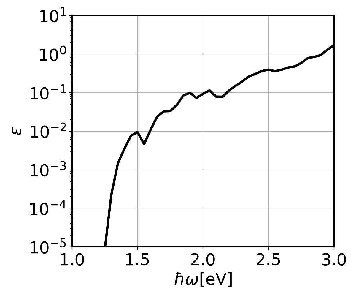
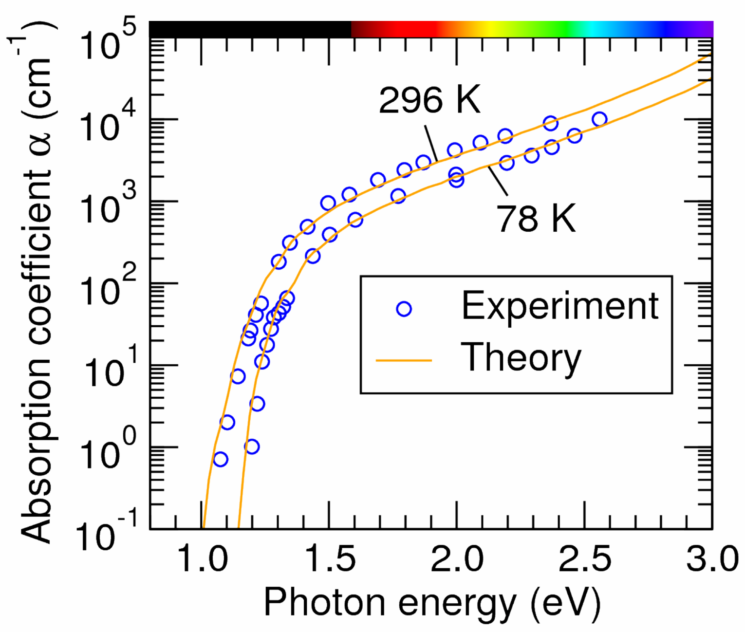
The fine \(\mathbf{k}\) and \(\mathbf{q}\) point grids need to be denser for production calculations. At convergence you should get a result similar to Fig. 3 of J. Noffsinger et al., Phys. Rev Lett. 108, 167402 (2012). Note that the relationship between Im \(\epsilon(\omega)\) and the absorption coefficient is \(\alpha(\omega)=\frac{\omega}{c n_r(\omega)}\text{Im }\epsilon(\omega)\). The paper assumes a constant refractive index of \(n_r=3.4\).

Action. Calculate free-carrier absorption (FCA)

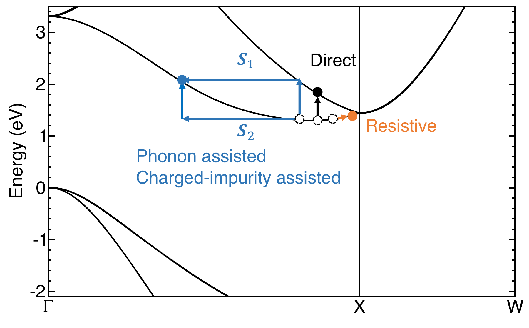
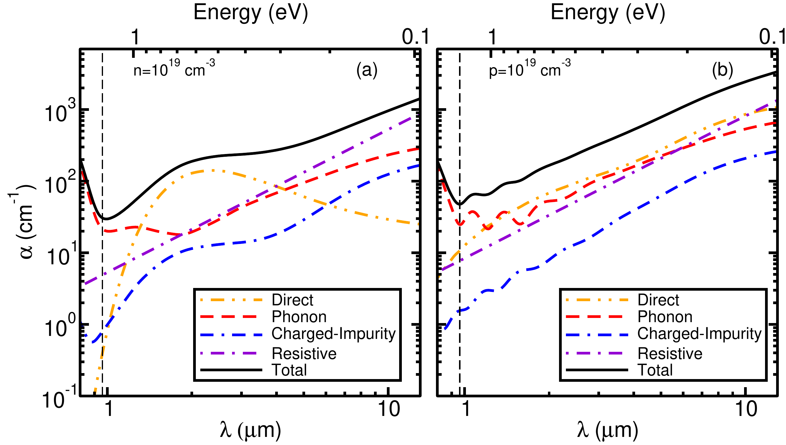
In addition to the phonon-assisted optical absorption, you can add the combination of tags carrier and ncarrier to specify the carrier density in n-type (positive ncarrier) or p-type (negative ncarrier) semiconductors to study phonon-assisted free-carrier absorption. Free-carrier absorption occurs in doped semiconductors/metals when the conduction band minimum or valence band maximum is partially occupied/empty. Various mechanisms need to be considered, as illustrated by Fig. 1 in Phys. Rev. B 106, 205203:

The input for such a calculation is provided in epw3.in. Note that some of the previous output epsilon files in epw2 will be overridden.

epw3.in

&inputepw
  ...

  omegamin = 0.05
  omegamax = 3.0
  omegastep = 0.05
  carrier   = .true.
  ncarrier  = 1e19

  ii_g = .true.
  ii_n = 1e19
  ii_lscreen = .true.

  sigma_ref = 20000

  ...

  nkf1        = 16
  nkf2        = 16
  nkf3        = 16
  nqf1        = 16
  nqf2        = 16
  nqf3        = 16

  ...
 /

The following tags are relevant for free-carrier absorption:

• carrier: enable calculation of free-carrier absorption. The Fermi level will be determined by the carrier density.

• ncarrier: free-carrier density in cm\(^{-3}\), positive for free electrons and negative for free holes.

• ii_g, ii_n, ii_lscreen: optical tags, enables calculation of ionized-impurity scattering matrix element (See tutorial Wed.7. ) to enable ionized-impurity assisted optics.

• sigma_ref: conductivity of the material in \(\Omega^{-1}\,\mathrm{m}^{-1}\). Used to determine the resistive contribution within a constant relaxation time approximation:

  \[\text{Im }\epsilon^{\mathrm{resis}}(\omega)=\frac{4 \pi \sigma}{\omega\left(1+\omega^2 \tau^2\right)}\]

Note that the \(\mathbf{k}\)- and \(\mathbf{q}\)-points grid are finer in the input for this optional calculation. Since free-carrier absorption happens close to the conduction band minimum or valence band maximum, a much denser grid is necessary to obtain converged result. In practice, similar to the case of mobility calculations, one can typically set fermi_energy close to the conduction band minimum (for free electrons) or valence band maximum (for free holes), and use a smaller value of fsthick to reduce the computational cost due to that free-carrier absorption is dominant only in sub-gap region where photon energy is relatively small compared to cross-gap indirect absorption. Note that in this case, fermi_energy is not used to set the Fermi-level used to calculate absorption, but only used to determine the states to consider according to fsthick.

We evaluate the free-carrier absorption in silicon:

$ ibrun -np 56 $PATHQE/bin/epw.x -npool 28 -nimage 2 < epw3.in > epw3.out

Several outputs will be generated when free-carrier absorption is enabled:

• epsilon2_indabs_300.0K.dat: Phonon-assisted contribution.

• epsilon2_indabs_imp_300.0K.dat: Ionized-impurity-assisted contribution.

• epsilon2_dirabs_300.0K.dat, Direct contribution.

• epsilon2_indabs_resis_300.0K.dat: Resistive contribution.

You may notice that the spectrum now has a strong dependence on the broadening \(\eta\) in the denominators of \(\mathbf{S}_1\) and \(\mathbf{S}_2\), which is due to the divergence of the denominator. This divergence is present when direct transition (in this case, inter-conduction bands) is possible, and is a limitation of the second-order perturbation theory itself. It can be reduced by numerical approaches to cancel the diverging term, see e.g. Brown et al., ACS Nano, 10.1, 957-966 (2016). Plot the direct, phonon-assisted, charged-impurity, and resistive contributions to the spectra:

python3 ../../py_codes/plot_fca.py

This will generate Si_fca.png:

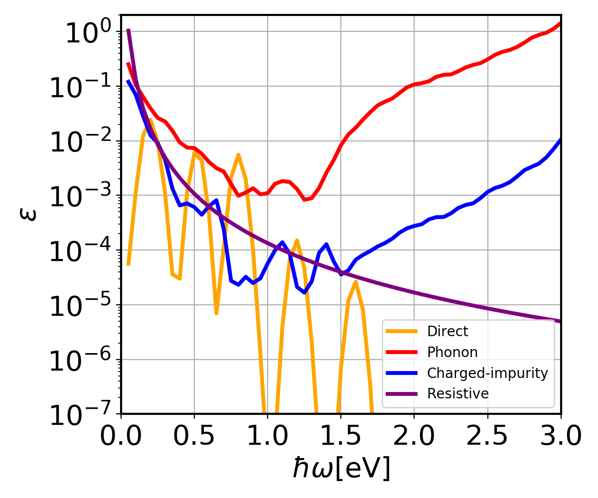
You will notice the \(\text{Im }\epsilon(\omega)\) from all the contributions now contain sub-gap contributions that result from free-carrier absorption. In addition, one can see a severe underconvergence for all the contributions due to Brillouin zone sampling. In our previous study, a grid of \(48\times48\times48\) was required for converged free-carrier absorption spectra of silicon. More details about free-carrier absorption can be found at: Phys. Rev. B 106, 205203. The converged result e.g. using a grid of \(48\times48\times48\), is similar to Fig. 2 in the paper (note that the x-axis in the paper is wavelength, i.e. \(\lambda_{\text{nm}}\approx1.24/(\hbar\omega)_{\text{eV}}\)):

1.4 Full spectra optical absorption with QDPT

In this step we are going to calculate the optical absorption of Si for full photon spectra Phys. Rev. B 109, 195127 (2024). We will learn the basic method to run a quasi-degenerate perturbation theory (QDPT) calculation.

Action. Do a restart calculation and compute the optical absorption spectrum of Si using QDPT.

Go to the QDPT/ folder to run these calculations. Like the previous step, we will restart the calculation from the si.epmatwp file.

$ cd ../QDPT/
$ ln -s ../dmedata.fmt ../ksdata.fmt ../si.ukk ../crystal.fmt \
        ../epwdata.fmt ../save/ ../si.epmatwp ../vmedata.fmt .

The input file is as follows:

epw2.in

&inputepw
prefix = 'si'            !Prefix used
amass(1) = 28.08         !Atomic mass
outdir = './'            !Output directory
elph = .true.            !Perform electron-phonon calculations
epwwrite = .false.       !Write epmatwp for restart
epwread = .true.         !Read epmatwp file and few others for restart
etf_mem = 1              !Optimization
nbndsub = 8              !Number of bands
asr_typ = 'crystal'      !Acoustic sum-rule
use_ws = .true.          !Should we use Wigner-Seitz cell
wannierize = .false.     !Wannierization
fsthick = 6.0            !Fermi surface thickness
degaussw = 0.1           !Gaussian spread (for DOS)
dvscf_dir = './save'     !dvscf directory
nk1 = 6                  !Coarse grid kx
nk2 = 6                  !Coarse grid ky
nk3 = 6                  !Coarse grid kz
nq1 = 3                  !Coarse grid qx
nq2 = 3                  !Coarse grid qy
nq3 = 3                  !Coarse grid qz

!!!!! Parameters of optical absorption !!!!!!

temps = 300.0            !Temperatures
loptabs = .true.         !For optical absorption
omegamin = 0.05          !Photon energy minimum
omegamax = 4.0           !Photon energy maximum
omegastep = 0.05         !Photon energy resolution
nkf1 = 12                !Fine grid kx
nkf2 = 12                !Fine grid ky
nkf3 = 12                !Fine grid kz
nqf1 = 3                 !Fine grid qx
nqf2 = 3                 !Fine grid qy
nqf3 = 3                 !Fine grid qz
mp_mesh_k = .true.       !Use IBZ
efermi_read = .true.     !Read Fermi level
fermi_energy = 6.2       !Fermi energy
/

• loptabs: enable calculation of direct and phonon-assisted optical absorption using quasi-degenerate perturbation theory.

$ ibrun -np 56 $PATHQE/bin/epw.x -npool 56 < epw2.in > epw2.out

Now, the calculation for QDPT starts. Here, we are calculating with \(12\times12\times12\) k grid and \(3\times3\times3\) q grid. The photon energy range is \(0-4.0\) eV. With this range we cover both the direct and indirect absorption regime for Si.

QDPT outputs the imaginary dielectric constant \(\epsilon_2(\omega)\) as a function of photon energy \(\hbar\omega\). The relevant equation is

\[\begin{split}\begin{aligned} && \varepsilon_2(\omega) = \frac{\pi e^2}{\epsilon_0 \Omega} \frac{1}{\omega^2}\frac{1}{N} \sum_{i_0,p} Z^{-1}\exp{(-\beta E_{i_0})} \nonumber \\ && \times\, \Bigg|\,\mathbf{e}\cdot \!\sum_{cv\mathbf{k}} \Bigg\{ U^*_{p,i_0-1_{v\mathbf{k}}+1_{c\mathbf{k}}} \mathbf{v}_{cv\mathbf{k}} \nonumber %\\ && +\,\,\,\,N^{-1/2} \sum_{\mathbf{q}\nu\eta} \sqrt{n_{\mathbf{q}\nu}\!+\!\frac{1+\eta}{2}} \,\, U^*_{p,i_0-1_{v\mathbf{k}}+1_{c\mathbf{k}+\mathbf{q}}+\eta 1_{-\eta \mathbf{q}\nu}} \nonumber \\ && \times \Bigg[ \sum_{c'} \frac{ g_{cc'\nu}(\mathbf{k},\mathbf{q}) \mathbf{v}_{c'v\mathbf{k}} } {(\bar E\!-\!E_{i_0})\!-\!(\varepsilon_{c'\mathbf{k}}\!-\!\varepsilon_{v\mathbf{k}})} \, \theta_{c'v\mathbf{k}} %\nonumber \\ %& & + \,\,\, \sum_{v'} \frac{ \mathbf{v}_{cv'\mathbf{k}+\mathbf{q}} \, g_{v'v\nu}(\mathbf{k},\mathbf{q}) } {(\bar E\!-\!E_{i_0})\!-\!(\varepsilon_{c\mathbf{k}+\mathbf{q}}\!-\!\varepsilon_{v'\mathbf{k}+\mathbf{q}})} \,\theta_{cv'\mathbf{k}+\mathbf{q}} \! \nonumber \\ & & + \,\,\, \sum_{c'} \frac{\mathbf{v}_{cc'\mathbf{k}+\mathbf{q}} \, g_{c'v\nu}(\mathbf{k},\mathbf{q}) }{\varepsilon_{v\mathbf{k}}\!-\!\varepsilon_{c'\mathbf{k}+\mathbf{q}}\!-\!\eta\hbar\omega_{-\eta\mathbf{q}\nu}} %\nonumber \\ %&& + \,\,\, \sum_{v'} \frac{g_{cv'\nu}(\mathbf{k},\mathbf{q}) \mathbf{v}_{v'v\mathbf{k}} } {\varepsilon_{v'\mathbf{k}}\!-\!\varepsilon_{c\mathbf{k}+\mathbf{q}}\!-\!\eta\hbar\omega_{-\eta\mathbf{q}\nu}} \Bigg] \!\Bigg\}\! \Bigg|^2 \nonumber \\ && \times\,\,\,\,\delta(E_p-E_{i_0}- \hbar \omega)~. \label{eq.eps.qd} \end{aligned}\end{split}\]

In this expression, the energy of the initial state \(|i_0\rangle\) is given by \(E_{i_0} = E_0 + \sum_{\mathbf{q}\nu} \hbar\omega_{\mathbf{q}\nu}/2 + \sum_{\mathbf{q}\nu} n_{\mathbf{q}\nu} \hbar\omega_{\mathbf{q}\nu}\), where \(E_0\) is the energy of the electronic ground state. The canonical average must be performed over all possible occupations \(n_{\mathbf{q}\nu} = 0,1,2,\cdots\). Unlike in second-order perturbation theory, in this case the transition rates are not simple linear functions of \(n_{\mathbf{q}\nu}\), therefore the replacement of \(n_{\mathbf{q}\nu}\) by the Bose-Einstein occupation is not allowed in principle. In particular, the occupations \(n_{\mathbf{q}\nu}\) are implicitly contained in the energies \(E_{i_0}\), in the unitary matrices \(U_{mp}\), and in the eigenvalues \(E_p\). The choice of occupations \(n_{\mathbf{q}\nu}\) is determined by flag nq_init .

nq_init = -1 (default) \(\rightarrow\) Bose-Einstein

nq_init = -3 \(\rightarrow\) Monte-Carlo integration of Eq. \(\epsilon_2(\omega)\) above.

From the imaginary dielectric constant, the absorption coefficient and luminescence can be calculated with simple expressions (see Phys. Rev. B 109, 195127 (2024)).

===================================================================
Phonon-assisted absorption with quasi-degenerate perturbation
===================================================================

Fermi surface thickness =   6.000000 eV

The following temperatures are calculated:

Temperature T =   0.025852 eV

size for cell = 270.169326 per A

nqtotf =         27

nktotf =         72

************************************************************************

            QDPT calculation accelerated with ELPA Library

Refer: https://elpa.mpcdf.mpg.de/ELPA_PUBLICATIONS.html for citation

************************************************************************

****************************************************

*****  Automatic generation of QDPT meshgrids  *****

 Number of QDPT meshgrids to be performed:         17

****************************************************
Size of QD bins    239.38meV
Finished building matrix

The key items to notice here are

1. The Fermi surface thickness which dictates up to what range the states are included for perturbation.

2. The temperature (300.0 K/ 25.852 meV)

3. QD bin size (automatically determined to 239.38 meV (ensures convergence))

4. Number of QD bins inside the photon energy range is 17

Further down the output,

Performing mesh =        15
Finished sorting, Entering eigenvalue calculation

QD array rank =        905

Building Hamiltonian with total elements:      1062

Starting diagonalization

LAPACK diagonalization complete

Used LAPACK for diagonalization

Performing epsilon summation

As stated, QDPT is a two-step process,

• In step 1: (starting diagonalization) we diagonalize the QD Hamiltonian in the QD bin

• In step 2: (performing epsilon summation) we perform the summation to obtain the \(\epsilon_2\) in the QDPT expression above

After the calculation ends:

python3 ../../py_codes/plot_contributions.py

This will generate Si_contribution.png:

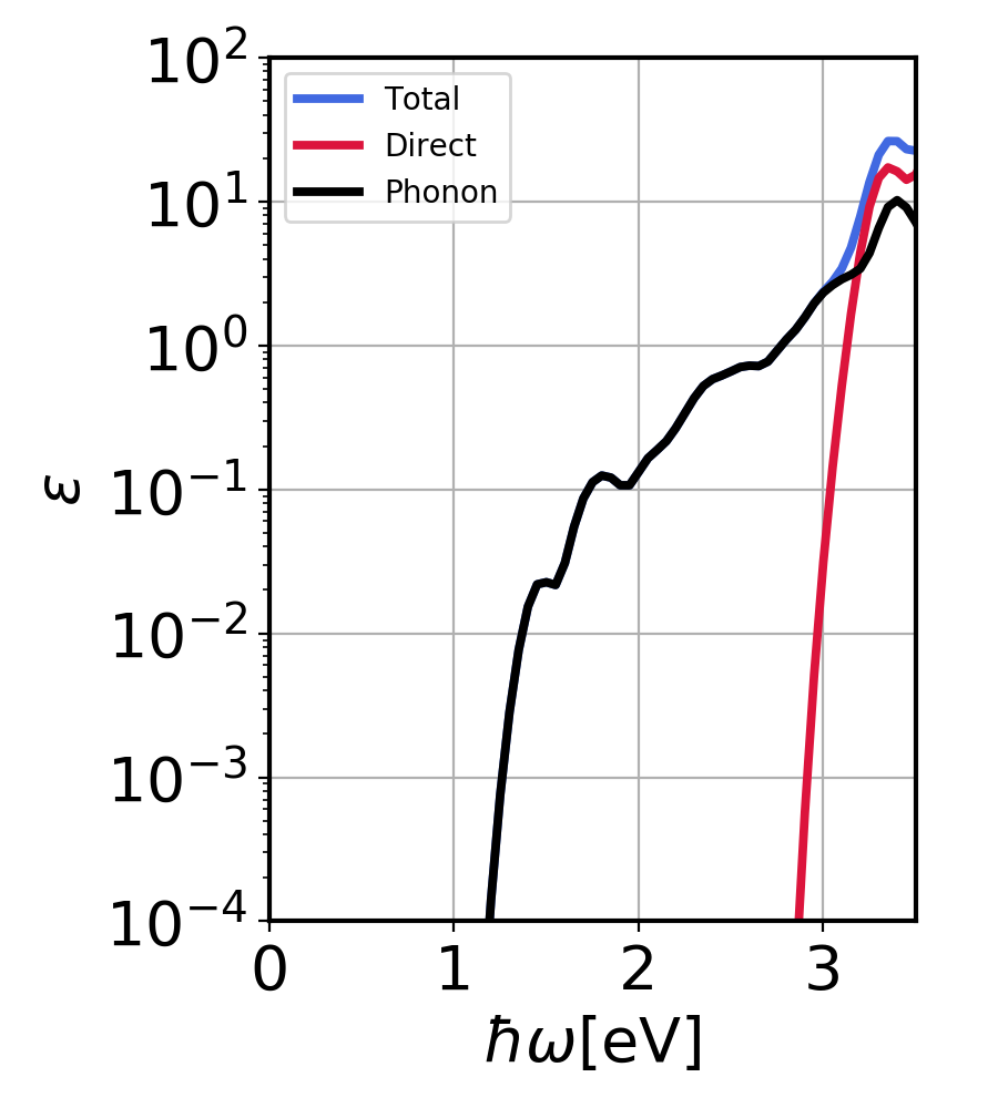
Silicon imaginary dielectric constant. Contributions from direct and phonon-assisted processes.

Here, we plot the silicon imaginary dielectric coefficient and its spectral decomposition in phonon and direct part. We see that below 3 eV (below direct gap) phonon-assisted process dominates, while after 3 eV, the direct contribution dominates.

These calculations are unconverged and a denser grid of \(60\times60\times60\) \(\mathbf{k}\)-grid would converge the calculation. After convergence the results would appear like,

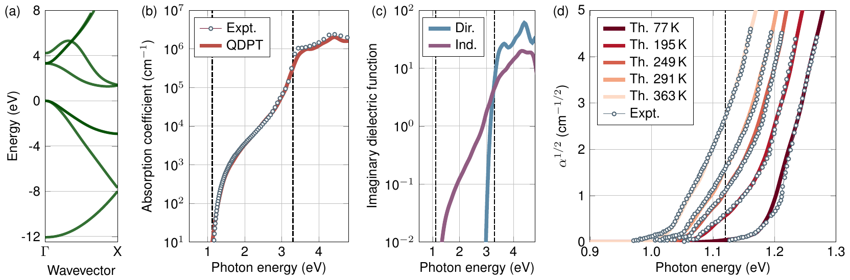
Silicon bandstructure(a), absorption coefficient (b), contributions from direct and phonon-assisted processes (c), absorption coefficient near the absorption edge (d). Taken verbatim from Phys. Rev. B 109, 195127 (2024)

Action. Save the calculation files.

$ cp epsilon2_indabs_300.0K_17.dat epsilon2_indabs_300.0K_all.dat

While for coarser grids, it is possible to run in one calculation, for denser grids, one has to perform restart calculations. In QDPT, the calculations are independent of the QD bin. Therefore, we can submit calculations independently for each QD bin.

We will perform two such calculations, first using epw2_15.in where we calculate up to QD bin 15. Next using epw2_17.in where we start from QD bin 16 and go up to 17 (2 bins). Finally, we sum the output using “py_eps_sum.py”

Action. Run the EPW restart calculation for QD bins 15 and 17.

epw2_15.in

&inputepw
prefix = 'si'            !Prefix used
amass(1) = 28.08         !Atomic mass
outdir = './'            !Output directory
elph = .true.            !Perform electron-phonon calculations
epwwrite = .false.       !Write epmatwp for restart
epwread = .true.         !Read epmatwp file and few others for restart
etf_mem = 1              !Optimization
nbndsub = 8              !Number of bands
asr_typ = 'crystal'      !Acoustic sum-rule
use_ws = .true.          !Should we use Wigner-Seitz cell
wannierize = .false.     !Wannierization
fsthick = 6.0            !Fermi surface thickness
degaussw = 0.1           !Gaussian spread (for DOS)
dvscf_dir = './save'     !dvscf directory
nk1 = 6                  !Coarse grid kx
nk2 = 6                  !Coarse grid ky
nk3 = 6                  !Coarse grid kz
nq1 = 3                  !Coarse grid qx
nq2 = 3                  !Coarse grid qy
nq3 = 3                  !Coarse grid qz

!!!!! Parameters of optical absorption !!!!!!

temps = 300.0            !Temperatures
loptabs = .true.         !For optical absorption
len_mesh = 18            !Number of QD bins
meshnum = 15             !Last QD bin
omegamin = 0.05          !Photon energy minimum
omegamax = 4.0           !Photon energy maximum
omegastep = 0.05         !Photon energy resolution
nkf1 = 12                !Fine grid kx
nkf2 = 12                !Fine grid ky
nkf3 = 12                !Fine grid kz
nqf1 = 3                 !Fine grid qx
nqf2 = 3                 !Fine grid qy
nqf3 = 3                 !Fine grid qz
mp_mesh_k = .true.       !Use IBZ
efermi_read = .true.     !Read Fermi level
fermi_energy = 6.2       !Fermi energy
/

epw2_17.in

&inputepw
prefix = 'si'            !Prefix used
amass(1) = 28.08         !Atomic mass
outdir = './'            !Output directory
elph = .true.            !Perform electron-phonon calculations
epwwrite = .false.       !Write epmatwp for restart
epwread = .true.         !Read epmatwp file and few others for restart
etf_mem = 1              !Optimization
nbndsub = 8              !Number of bands
asr_typ = 'crystal'      !Acoustic sum-rule
use_ws = .true.          !Should we use Wigner-Seitz cell
wannierize = .false.     !Wannierization
fsthick = 6.0            !Fermi surface thickness
degaussw = 0.1           !Gaussian spread (for DOS)
dvscf_dir = './save'     !dvscf directory
nk1 = 6                  !Coarse grid kx
nk2 = 6                  !Coarse grid ky
nk3 = 6                  !Coarse grid kz
nq1 = 3                  !Coarse grid qx
nq2 = 3                  !Coarse grid qy
nq3 = 3                  !Coarse grid qz

!!!!! Parameters of optical absorption !!!!!!

temps = 300.0            !Temperatures
loptabs = .true.         !For optical absorption
len_mesh = 18            !Number of QD bins
meshnum = 17             !Last QD bin
start_mesh = 16          !First QD bin
omegamin = 0.05          !Photon energy minimum
omegamax = 4.0           !Photon energy maximum
omegastep = 0.05         !Photon energy resolution
nkf1 = 12                !Fine grid kx
nkf2 = 12                !Fine grid ky
nkf3 = 12                !Fine grid kz
nqf1 = 3                 !Fine grid qx
nqf2 = 3                 !Fine grid qy
nqf3 = 3                 !Fine grid qz
mp_mesh_k = .true.       !Use IBZ
efermi_read = .true.     !Read Fermi level
fermi_energy = 6.2       !Fermi energy
/

$ ibrun -np 56 $PATHQE/bin/epw.x -npool 56 < epw2_15.in > epw2_15.out
$ ibrun -np 56 $PATHQE/bin/epw.x -npool 56 < epw2_17.in > epw2_17.out

After these calculations finish, they produce two epsilon2 files with *_15.dat and *_17.dat. These files contain the imaginary dielectric constant. We sum them using a python code (py_sum_eps.py).

python3 ../../py_codes/py_sum_eps.py

Now, plot all four using plot_all.py

python3 ../../py_codes/plot_epsilon_all.py

This will generate Si.png:

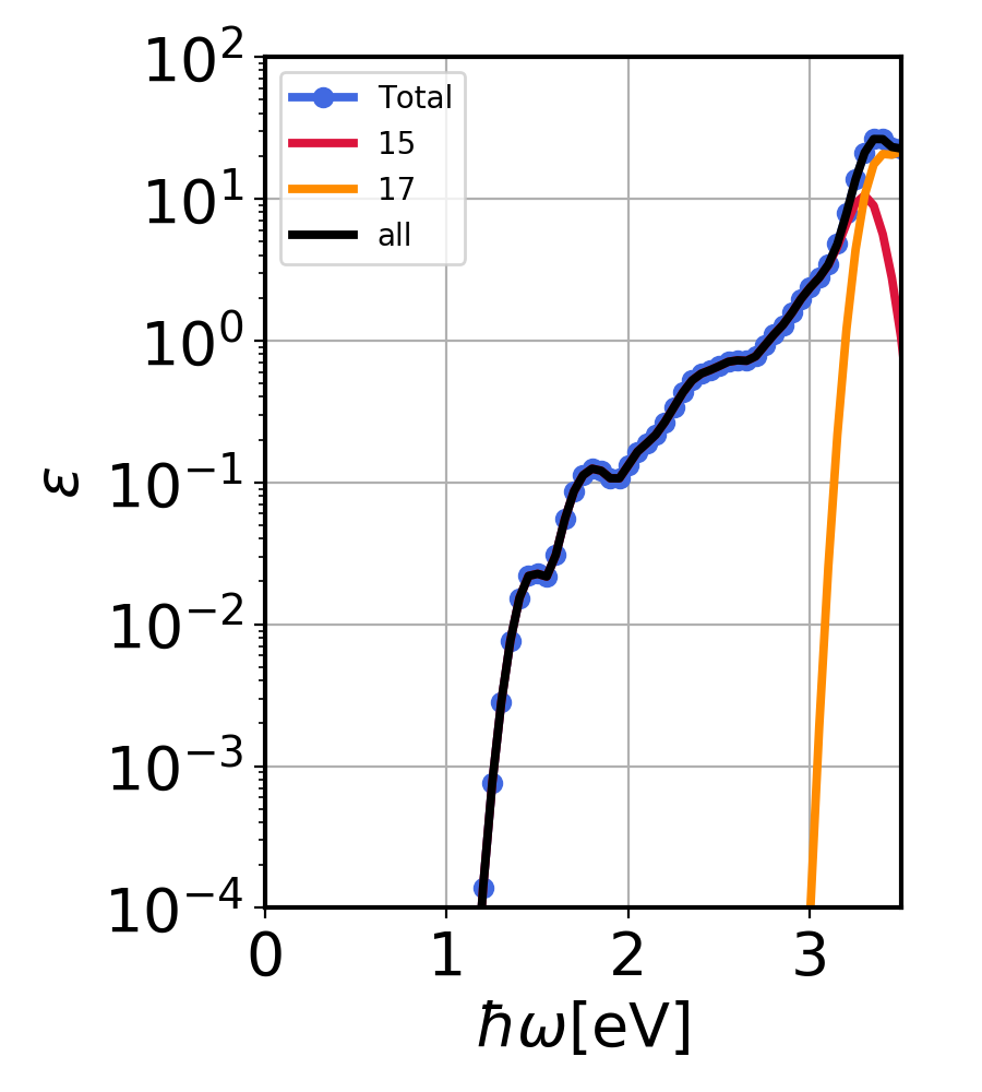
Silicon imaginary dielectric constant for sum of QD bins 15 and 17 (blue), individual, (red and orange) and the single calculation with both bins. (black).

In the above figure, you see the silicon imaginary dielectric constant for sum of QD bins 15 and 17 (blue), individual, (red and orange) and the single calculation with both bins. (black). As you can see, adding the imaginary dielectric constant from both the bins amounts to calculating them in one single calculation.

Exercise 2: Optical absorption in GaAs

In this example we are going to calculate the optical absorption in GaAs (a direct gap material) for full photon spectra Phys. Rev. B 109, 195127 (2024).

$ cd ../../exercise2/

2.1 Preliminary calculations with Quantum Espresso

Action. Run a self-consistent calculation on a homogeneous \(6\times6\times6\) \(\mathbf{k}\)-point grid and a phonon calculation on a homogeneous \(3\times3\times3\) \(\mathbf{q}\)-point grid, and a uniform \(\mathbf{k}\)-grid calculation on a grid of \(6\times6\times6\) using the following input files (scf.in, ph.in, and nscf.in):

scf.in

&CONTROL
calculation = 'scf'
verbosity = 'high'
restart_mode = 'from_scratch'
outdir = './'
pseudo_dir = './pseudos'
prefix = 'GaAs'
/
&SYSTEM
ibrav = 0
nat = 2
ntyp = 2
ecutwfc = 60
ecutrho = 240
/
&ELECTRONS
conv_thr = 1E-11
diagonalization = 'david'
/
ATOMIC_SPECIES
Ga 95.95 Ga.upf
As 32.06 As.upf
ATOMIC_POSITIONS crystal
Ga 0.25 0.25 0.25
As 0.0 0.0 0.0

K_POINTS automatic
6 6 6 0 0 0

CELL_PARAMETERS angstrom
0.0  2.86759328207563  2.86759328207563
2.86759328207563  0.0  2.86759328207563
2.86759328207563  2.86759328207563  0.0

ph.in

&inputph
prefix = 'GaAs'
fildyn = 'GaAs.dyn'
ldisp = .true.
fildvscf = 'dvscf'
nq1 = 3
nq2 = 3
nq3 = 3
tr2_ph = 1.0d-14
/

nscf.in

&CONTROL
calculation = bands
verbosity = 'high'
restart_mode = 'from_scratch'
outdir = './'
pseudo_dir = './pseudos'
prefix = 'GaAs'
/
&SYSTEM
ibrav = 0
nat = 2
ntyp = 2
ecutwfc = 60
ecutrho = 240
nbnd = 36
/
&ELECTRONS
conv_thr = 1E-11
diagonalization = 'david'
/
ATOMIC_SPECIES
Ga 95.95 Ga.upf
As 32.06 As.upf
ATOMIC_POSITIONS crystal
Ga 0.25 0.25 0.25
As 0.0 0.0 0.0

K_POINTS crystal
 216
0.000 0.000 0.000 0.00463
0.000 0.000 0.167  0.00463
  ...

$ ibrun -np 8 $PATHQE/bin/pw.x -npool 8 < scf.in > scf.out
$ ibrun -np 56 $PATHQE/bin/ph.x -npool 28 < ph.in > ph.out
$ ibrun -np 8 $PATHQE/bin/pw.x -npool 8 < nscf.in > nscf.out

Action. Run the python post-processing to create the save folder (No job submission needed, can be run simply on the login node.)

$  python3 $PATHQE/EPW/bin/pp.py

The script will ask you to enter the prefix used for the calculation. In this case enter “GaAs”. The script will create a new folder called “save” that contains the dvscf potential files, pattern files, and dynamical matrices on the IBZ.

2.2 Interpolation of the electron-phonon matrix elements with EPW

Action. Run the EPW calculation to obtain the electron-phonon matrix in Wannier representation using epw1.in.

epw1.in

&inputepw
prefix = 'GaAs'
amass(1) = 95.95
amass(2) = 32.06
outdir = './'
elph = .true.
epbwrite = .false.
epbread = .false.
epwwrite = .true.
epwread = .false.
etf_mem = 1
nbndsub = 8
asr_typ = 'crystal'
use_ws = .true.
wannierize = .true.
num_iter = 5000
iprint = 2
dis_win_max = 20
dis_froz_max = 10
fsthick = 1.2
temps = 1
degaussw = 0.005
dvscf_dir = './save'
band_plot = .true.
nk1 = 6
nk2 = 6
nk3 = 6
nq1 = 3
nq2 = 3
nq3 = 3
wdata(1) = 'guiding_centres = .true.'
wdata(2) = 'dis_num_iter = 500'
wdata(3) = 'num_print_cycles  = 10'
wdata(4) = 'dis_mix_ratio = 1'
wdata(5) = 'use_ws_distance = T'
dis_froz_min = -7
dis_win_min = -10
proj(1) = 'Ga : sp3'
proj(2) = 'As: sp3'
filkf = 'LGX.txt'
filqf = 'LGX.txt'
eig_read = false
/

$ ibrun -np 56 $PATHQE/bin/epw.x -npool 28 -nimage 2 < epw1.in > epw1.out

With the above input, we are instructing EPW to represent electron-phonon coupling in Wannier representation. Notice the starting Wannier orbitals.

Next, plot the bands using the Python scripts provided in py_codes:

$ python3 ../py_codes/plot_band_GaAs.py

The resulting band structure should look similar to the following:

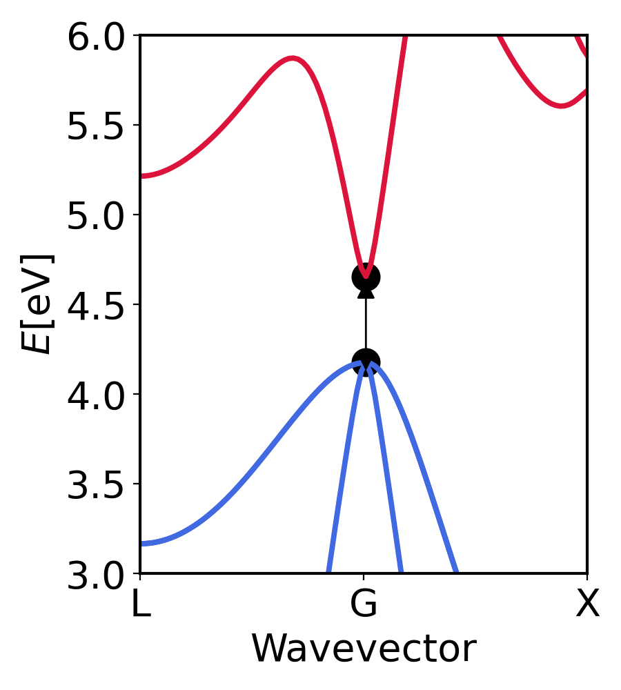
GaAs bandstructure. The arrow shows the minima of conduction band and maxima of valence band. We see that the gap is about 0.6 eV at the same k-point.

We see that the gap is about 0.6 eV which is lower than experimental gap of (1.4 eV). The reason is that PBE (GGA) underestimates the gap. It can be corrected by using GW eigenvalues as shown in the indabs tutorial.

2.3 Full spectra optical absorption with QDPT

Action. Run the EPW QDPT calculation, restarting from the GaAs.epmatwp electron-phonon matrix file.

epw2.in

&inputepw
prefix = 'GaAs'
amass(1) = 95.95
amass(2) = 32.06
outdir = './'
elph = .true.
epwwrite = .false.
epwread = .true.
etf_mem = 1
nbndsub = 8
asr_typ = 'crystal'
use_ws = .true.
wannierize = .false.
fsthick = 6.0
degaussw = 0.12
dvscf_dir = './save'
nk1 = 6
nk2 = 6
nk3 = 6
nq1 = 3
nq2 = 3
nq3 = 3
eig_read = .false.
loptabs = .true.

omegamin = 0.05        !Photon energy minimum
omegamax = 2.6         !Photon energy maximum
omegastep = 0.05       !Photon energy resolution
nkf1 = 36              !Fine grid kx
nkf2 = 36              !Fine grid ky
nkf3 = 36              !Fine grid kz
nqf1 = 3               !Fine grid qx
nqf2 = 3               !Fine grid qy
nqf3 = 3               !Fine grid qz
mp_mesh_k = .true.     !Use IBZ
efermi_read = .true.   !Read Fermi level
fermi_energy = 4.5     !Fermi energy
mode_res = 6           !Number of modes over which epsilon2 is decomposed
/

$ ibrun -np 56 $PATHQE/bin/epw.x -npool 56 < epw2.in > epw2.out

Notice, we have added an extra tag, mode_res. This tag controls among how many modes we spectrally decompose the imaginary dielectric constant. The maximum number of modes a system can have is \(3N\) where \(N\) is the number of atoms. Hence, for GaAs we have maximum number of modes \(= 6\).

After the calculation finishes, perform

$ python3 ../py_codes/plot_epsilon_GaAs.py

This will generate GaAs.png:

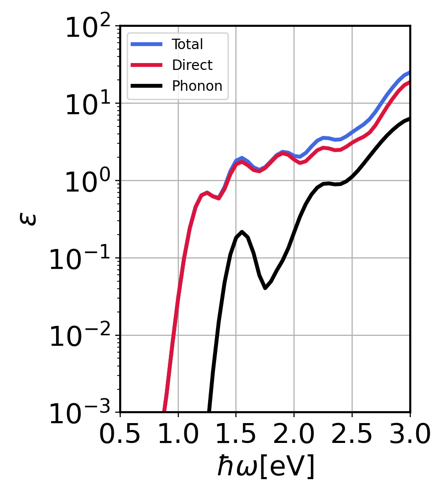
GaAs imaginary dielectric constant. Contributions from direct and phonon-assisted processes.

We see that the phonon-assisted contribution remains below direct contribution since GaAs is direct gap material. However, with increasing photon energy, we see an increase in phonon contribution. This happens because the phase-space increases for phonon assisted processes.

We next plot the mode resolved imaginary dielectric constant. To do so

$ python3 ../py_codes/plot_epsilon_GaAs_cont.py

This will generate GaAs_contribution.png:

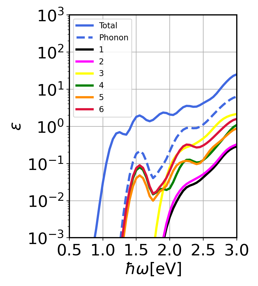
GaAs imaginary dielectric constant. Contributions from direct and phonon-assisted processes.

With this we can see the contribution from each of the phonon modes to the imaginary dielectric constant.

Exercise 3: Si QDPT convergence (Optional)

This is a bonus exercise. In this exercise we are going to understand the convergence of QDPT calculation with respect to QD bin size.

$ cp ../exercise3/*.in ../exercise1/QDPT/
$ cd ../exercise1/QDPT/

Notice, inside exercise3 you will find 4 .in files, epw2_0.35.in, epw2_0.45.in, epw2_2.80.in, and epw2_all.in. Here the number after _ corresponds to respective QD bin size.

epw2_0.35.in

&inputepw
prefix = 'si'           !Prefix used
amass(1) = 28.08         !Atomic mass
outdir = './'            !Output directory
elph = .true.            !Perform electron-phonon calculations
epwwrite = .false.       !Write epmatwp for restart
epwread = .true.         !Read epmatwp file and few others for restart
etf_mem = 1              !Optimization
nbndsub = 8              !Number of bands
asr_typ = 'crystal'      !Acoustic sum-rule
use_ws = .true.          !Should we use Wigner-Seitz cell
wannierize = .false.     !Wannierization
fsthick = 6.0            !Fermi surface thickness
degaussw = 0.1           !Gaussian spread (for DOS)
dvscf_dir = './save'     !dvscf directory
nk1 = 6                  !Coarse grid kx
nk2 = 6                  !Coarse grid ky
nk3 = 6                  !Coarse grid kz
nq1 = 3                  !Coarse grid qx
nq2 = 3                  !Coarse grid qy
nq3 = 3                  !Coarse grid qz

!!!!! Parameters of optical absorption !!!!!!

temps = 300.0            !Temperatures
loptabs = .true.         !For optical absorption
QD_bin = 0.35            !QD bin size
QD_min = 0.6             !QD bin starting energy
omegamin = 0.05          !Photon energy minimum
omegamax = 4.0           !Photon energy maximum
omegastep = 0.05         !Photon energy resolution
nkf1 = 12                !Fine grid kx
nkf2 = 12                !Fine grid ky
nkf3 = 12                !Fine grid kz
nqf1 = 3                 !Fine grid qx
nqf2 = 3                 !Fine grid qy
nqf3 = 3                 !Fine grid qz
mp_mesh_k = .true.       !Use IBZ
efermi_read = .true.     !Read Fermi level
fermi_energy = 6.2       !Fermi energy
/

Notice, the tag QD_bin which dictates the size of QD bin in eV. Here it is \(350\) meV.

Action. Now we perform the QDPT calculation for two of the three input files.

$ ibrun -np 56 $PATHQE/bin/epw.x -npool 56 < epw2_0.45.in > epw2_0.45.out
$ ibrun -np 56 $PATHQE/bin/epw.x -npool 56 < epw2_0.35.in > epw2_0.35.out

After this calculation finishes, there will be two extra epsilon2_indabs files with subscript 8 and 10. We now plot the imaginary dielectric constant from these calculations and compare with automatic QD bin generation (epsilon2_indabs_300.0K_all.dat).

$ python3 ../../py_codes/plot_convergence.py

This will generate Si_conv.png.

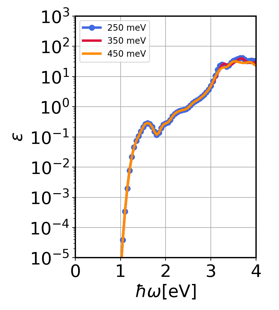
Si imaginary dielectric constant calculated using QDPT for three QD bins.

We see the QD bin generated automatically ensures convergence. However, for each material, this convergence should be checked for production level calculations.

Something you can try in free time after school.

Action. Now perform the same calculations with file epw2_2.80.in

Note: For this calculation you need to submit over 4 nodes. Also, this calculation will take longer (about 40 minutes), so try at home!

$ ibrun -np 56 $PATHQE/bin/epw.x -npool 56 < epw2_2.80.in > epw2_2.80.out
$ ibrun -np 56 $PATHQE/bin/epw.x -npool 56 < epw2_all.in > epw2_all.out

After these calculations finish, they produce two epsilon2 files *_2.dat and *_17.dat.

The epw2_all.in file is a simple QDPT calculation with automatic QD bin but with a denser \(\mathbf{q}\)-grid of \(6\times6\times6\). While the epw2_2.80.in is a QDPT calculation with a QD bin of size 2800 meV. This large size ensures we are performing full-diagonalization (almost).

Plot them using

$ python3 ../../py_codes/plot_convergence2.py

This will generate Si_conv2.png.

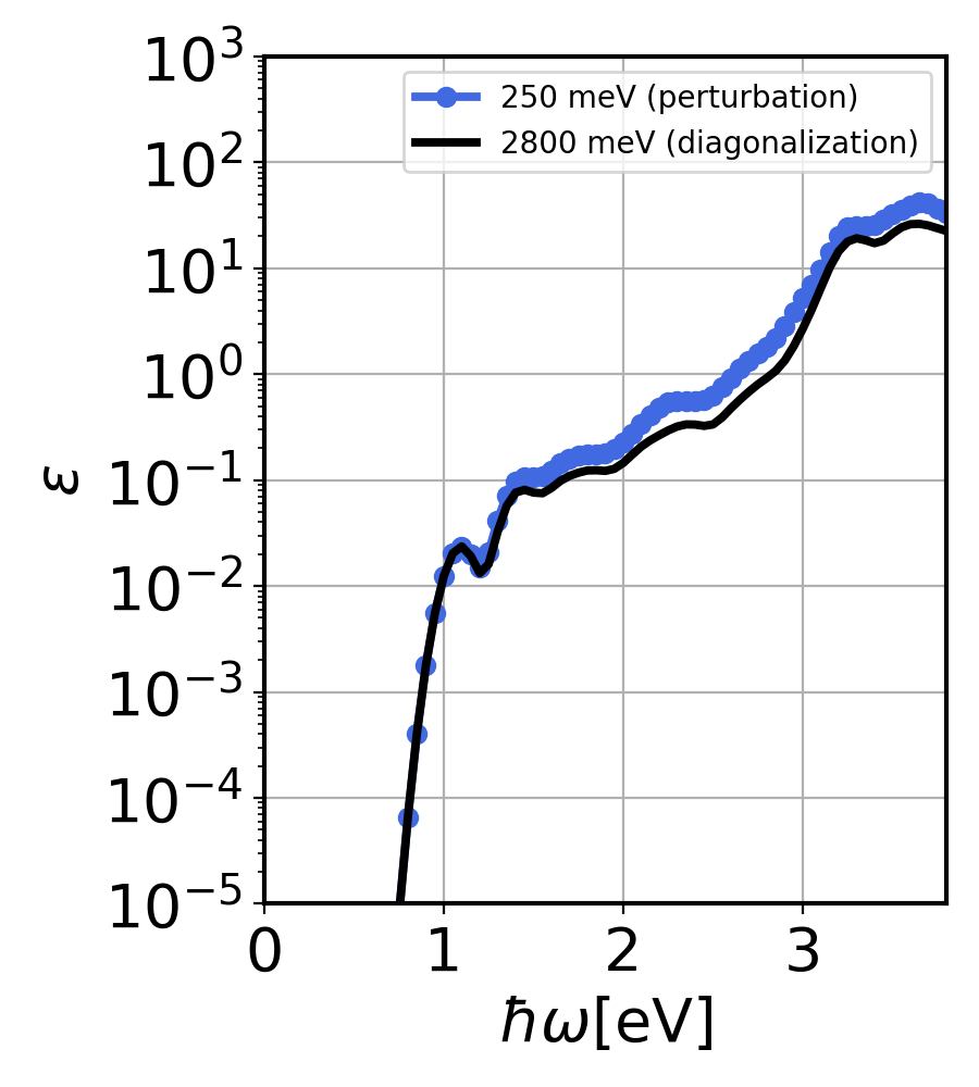
Si imaginary dielectric constant calculated using QDPT for two QD bins. Here, at size 2800 meV, we almost reach full diagonalization.

As you can see, the perturbation and exact diagonalization give almost the same result. Slight difference is due to small grid sizes used and denser grids ensure exact comparison.

[1]

Note that direct absorption within the independent particle approximation is also calculated, see epsilon2_dirabs_300.0K.dat and epsilon2_dirabs_lorenz300.0K.dat. Careful convergence with respect to \(\mathbf{k}\)-grid is important.