Boltzmann transport equation¶

Alvaro Carrasco Alvarez 08/05/2026
Samuel Poncé and Viet-Anh Ha (2024)

Note

Hands-on based on Quantum ESPRESSO v7.6 and EPW v6.1.

Introduction¶

In this tutorial, we will show how to compute the resistivity of metals and the drift and hall mobility of semiconductors.

You are advised to prepare the following script file, e.g. run.sh:

run.sh

#!/bin/bash
#SBATCH -J job.ph # Job name
#SBATCH -N 1 # Total # of nodes
#SBATCH --ntasks-per-node 56
#SBATCH -t 01:00:00 # Run time (hh:mm:ss)
#SBATCH -A DMR23048
#SBATCH -p normal
#SBATCH --reservation=MATCSSI_Norm_June19

# Load packages
module load hdf5/1.10.4

# Launch MPI code...
export PATHQE=/work2/05193/sabyadk/shared/EPW_6.1s/q-e/

ibrun -n 56 $PATHQE/bin/pw.x -in scf.in -nk 8 1> scf.out 2> error.out
ibrun -n 56 $PATHQE/bin/ph.x -in ph.in -nk 8 1> ph.out 2> error.out

Note: You should update the script accordingly to each step of the tutorial. For the description for all input flags please follow the link:

EPW input documentation

To run each of the steps shown below, copy the script into the working folder and submit the job using:

$ sbatch run.sh

Action: To run the post-processing commands on the login node, we need to define the path to the post-processing scripts. Run the following commands to define the shortcut to the scripts:

$ module load hdf5/1.10.4
$ export PATHQE=/work2/05193/sabyadk/shared/EPW_6.1s/q-e

The first exercise is a tutorial on carrier transport including drift, Hall and impurity scattering and is considered as the basic tutorial. Exercise 2 shows the example of 2D materials, while Exercise 3 shows the case of carrier transport in metals and in magnetic systems (collinear magentism)

Exercise 1¶

1.1 Theory¶

In this example we are going to calculate the drift and Hall hole carrier mobility of c-BN. The drift mobility is obtained with:

\[\begin{aligned} \mu^{\mathrm{d}}_{\alpha\beta} = \frac{-1}{V_{\mathrm{uc}}n_{\text{c}}} \sum_n \int \frac{\mathrm{d}^3 k}{\Omega_{\mathrm{BZ}}} \, v_{n\mathbf{k}\alpha} \partial_{E_{\beta}} f_{n\mathbf{k}}, \end{aligned}\]

where the out of equilibrium occupations are obtained by solving the Boltzmann transport equation (BTE):

(1)¶\[ \begin{align}\begin{aligned}\begin{split}\begin{aligned} \partial_{E_{\beta}} f_{n\mathbf{k}} = ev_{n\mathbf{k}\beta}\frac{\partial f_{n\mathbf{k}}}{\partial\varepsilon_{n\mathbf{k}}}\tau_{n\mathbf{k}} + \frac{2\pi\tau_{n\mathbf{k}}}{\hbar}\sum_{m\nu}\int\frac{d^3q}{\Omega_{\mathrm{BZ}}}|g_{mn\nu}(\mathbf{k},\mathbf{q})|^2\big[(n_{\mathbf{q}\nu}+1-f_{n\mathbf{k}})\delta(\varepsilon_{n\mathbf{k}}-\varepsilon_{m\mathbf{k+q}}+\hbar\omega_{\mathbf{q}\nu})\nonumber\\ + (n_{\mathbf{q}\nu}+f_{n\mathbf{k}})\delta(\varepsilon_{n\mathbf{k}}-\varepsilon_{m\mathbf{k+q}}-\hbar\omega_{\mathbf{q}\nu})\big] \partial_{E_{\beta}} f_{m\mathbf{k+q}},\end{split}\\\end{aligned}\end{aligned}\end{align} \]

where the scattering rate in Eq. (1) is defined as:

(2)¶\[ \begin{align}\begin{aligned}\begin{split}\begin{aligned} \tau^{-1}_{n\mathbf{k}} = \frac{2\pi}{\hbar}\sum_{m\nu}\int\frac{\mathrm{d}^3q}{\Omega_\mathrm{BZ}}|g_{mn\nu}(\mathbf{k},\mathbf{q})|^2\big[(n_{\mathbf{q}\nu}+1-f_{n\mathbf{k}})\delta(\varepsilon_{n\mathbf{k}}-\varepsilon_{m\mathbf{k+q}}+\hbar\omega_{\mathbf{q}\nu}) \nonumber \\+ (n_{\mathbf{q}\nu}+f_{n\mathbf{k}})\delta(\varepsilon_{n\mathbf{k}}-\varepsilon_{m\mathbf{k+q}}-\hbar\omega_{\mathbf{q}\nu})\big].\end{split}\\\end{aligned}\end{aligned}\end{align} \]

A common approximation to Eq. (1) is called the self-energy relaxation time approximation (SERTA) and consists in neglecting the second term in the right-hand of the equation which gives:

\[\begin{aligned} \mu^{\mathrm{SERTA}}_{\alpha\beta} = \frac{-e}{V_{\mathrm{uc}}n_{\text{c}}} \sum_n \int \frac{\mathrm{d}^3 k}{\Omega_{\mathrm{BZ}}} \frac{\partial f_{n\mathbf{k}}}{\partial\varepsilon_{n\mathbf{k}}} v_{n\mathbf{k}\alpha}v_{n\mathbf{k}\beta}\tau_{n\mathbf{k}}. \end{aligned}\]

The low-field phonon-limited carrier mobility in the presence of a small finite magnetic field B is given by:

\[\begin{aligned} \mu_{\alpha\beta}(B_\gamma) = \frac{-1}{V_{\mathrm{uc}}n_{\text{c}}} \sum_n \int \frac{\mathrm{d}^3 k}{\Omega_{\mathrm{BZ}}} \, v_{n\mathbf{k}\alpha} [\partial_{E_{\beta}} f_{n\mathbf{k}}(B_\gamma) -\partial_{E_{\beta}} f_{n\mathbf{k}}], \end{aligned}\]

again solving the BTE with finite (small) magnetic field:

\[\begin{split}\begin{aligned} \big[1 - \frac{e}{\hbar}\tau_{n\mathbf{k}}(\mathbf{v}_{n\mathbf{k}}\times\mathbf{B})\cdot\nabla_\mathbf{k}\big]\partial_{E_\beta}f_{n\mathbf{k}}(B_\gamma) = ev_{n\mathbf{k}\beta}\frac{\partial f_{n\mathbf{k}}}{\partial\varepsilon_{n\mathbf{k}}}\tau_{n\mathbf{k}}+\frac{2\pi\tau_{n\mathbf{k}}}{\hbar}\sum_{m\nu}\int\frac{\mathrm{d}^3q}{\Omega_\mathrm{BZ}}|g_{mn\nu}(\mathbf{k},\mathbf{q})|^2\nonumber\\ \times\big[(n_{\mathbf{q}\nu}+1-f_{n\mathbf{k}})\delta(\varepsilon_{n\mathbf{k}}-\varepsilon_{m\mathbf{k+q}}+\hbar\omega_{\mathbf{q}\nu}) +(n_{\mathbf{q}\nu}+f_{n\mathbf{k}})\delta(\varepsilon_{n\mathbf{k}}-\varepsilon_{m\mathbf{k+q}}-\hbar\omega_{\mathbf{q}\nu})\big]\partial_{E_\beta}f_{m\mathbf{k+q}}(B_\gamma). \end{aligned}\end{split}\]

The Hall factor and Hall mobility are then obtained as:

\[\begin{split}\begin{aligned} r_{\alpha\beta} = \lim_{\mathbf{B}\rightarrow0}\sum_{\delta\epsilon}\frac{(\mu^\mathrm{d}_{\alpha\delta})^{-1}\mu_{\delta\epsilon}(\mathbf{B}) (\mu^\mathrm{d}_{\epsilon\beta})^{-1}}{|\mathbf{B}|},\\ \mu^\mathrm{Hall}_{\alpha\beta}(\hat{\mathbf{B}}) = \sum_{\gamma}\mu^\mathrm{d}_{\alpha\gamma}r_{\gamma\beta}(\hat{\mathbf{B}}), \end{aligned}\end{split}\]

where $\hat{\mathbf{B}}$ is the direction of the magnetic field. More information can be found in the review Rep. Prog. Phys. 83, 036501 (2020).

1.2 Preliminary calculations with Quantum ESPRESSO¶

First download the exercise files:

$ wget --content-disposition "https://drive.google.com/uc?export=download&id=1lxb7Uh0xV1Hlmv1XaUqnhyxLpMnpryAs"
$ tar -xvf Fri.4.CarrascoAlvarez.tar
$ cd Fri.4.CarrascoAlvarez/exercise1/

Action: Make a self-consistent calculation for c-BN.

scf.in

 &control
    calculation     = 'scf'
    prefix          = 'bn'
    restart_mode    = 'from_scratch'
    pseudo_dir      = '../pseudo/'
    outdir          = './'
 /
 &system
    ibrav           = 2
    celldm(1)       = 6.833
    nat             = 2
    ntyp            = 2
    ecutwfc         = 40
 /
 &electrons
    diagonalization = 'david'
    mixing_beta     = 0.7
    conv_thr        = 1.0d-13
 /
ATOMIC_SPECIES
  B  10.811   B-PBE.upf
  N  14.0067  N-PBE.upf
ATOMIC_POSITIONS {crystal}
 B    0.00  0.00   0.00
 N   -0.25  0.75  -0.25
K_POINTS automatic
8 8 8 0 0 0

Note: In practice the k-point grid needs to be fairly large in order to get converged dielectric function and Born effective charges during the following phonon calculation.

$ ibrun -n 56 $PATHQE/bin/pw.x -in scf.in -nk 8  1> scf.out 2> error.out

Action: Compute the vibrational properties of c-BN on a coarse 4$\times$4$\times$4 $\mathbf{q}$-point grid.

ph.in

&inputph
  tr2_ph=1.0d-17,
  prefix='bn',
  amass(1)=10.811,
  amass(2)=14.0067,
  outdir='./',
  fildyn='bn.dyn.xml',
  fildvscf='dvscf'
  ldisp=.true.,
  epsil=.true.,
  nq1 = 4,
  nq2 = 4,
  nq3 = 4
/

Note: We have the input variable epsil=.true. which computes the macroscopic dielectric constant in non-metallic systems. If you add .xml after the name of the dynamical matrix file, it will produce the data in XML format (preferred).
Note 2: The input variable responsible to produce the electron-phonon matrix element is fildvscf. Always make sure that this variable is present.
Note 3: Notice the very tight tr2_ph threshold parameter on the self-consistent first-order perturbed wavefunction. This is crucial to obtain good vibrational properties.

$ ibrun -n 56 $PATHQE/bin/ph.x -in ph.in -nk 8 1> ph.out 2> error.out

The calculation should take about 1 minute on 56 cores. During the run, notice the IBZ q-point grid:

Dynamical matrices for ( 4, 4, 4)  uniform grid of q-points
(   8 q-points):
  N         xq(1)         xq(2)         xq(3)
 0.000000000   0.000000000   0.000000000
-0.250000000   0.250000000  -0.250000000
 0.500000000  -0.500000000   0.500000000
 0.000000000   0.500000000   0.000000000
 0.750000000  -0.250000000   0.750000000
 0.500000000   0.000000000   0.500000000
 0.000000000  -1.000000000   0.000000000
-0.500000000  -1.000000000   0.000000000

as well as the dielectric function and Born effective charge tensor:

    Dielectric constant in cartesian axis

    (       4.597202520       0.000000000      -0.000000000 )
    (      -0.000000000       4.597202520      -0.000000000 )
    (      -0.000000000       0.000000000       4.597202520 )

    Effective charges (d Force / dE) in cartesian axis without acoustic sum rule applied (asr)

     atom    1  B     Mean Z*:        1.89176
Ex  (        1.89176        0.00000        0.00000 )
Ey  (        0.00000        1.89176        0.00000 )
Ez  (        0.00000       -0.00000        1.89176 )
     atom    2  N     Mean Z*:       -1.89376
Ex  (       -1.89376       -0.00000        0.00000 )
Ey  (       -0.00000       -1.89376       -0.00000 )
Ez  (        0.00000       -0.00000       -1.89376 )

The experimental dielectric constant in c-BN is about 4.46. More accurate values can be obtained with larger $\mathbf{k}$-point grids. c-BN is a polar material and has a Born effective charge of 1.89 which is very close to the converged theoretical value of 1.91.

Finally, we need to post-process some of the data to make it ready for EPW. To do so, we can use a python script. For inline scripts we need to load also the hdf5 module first

$ module load hdf5/1.10.4

Action: Run the python post-processing to create the save folder

$ python3 $PATHQE/EPW/bin/pp.py

The script will ask you to enter the prefix used for the calculation. In this case enter ”bn”. The script will create a new folder called ”save” that contains the dvscf potential files, pattern files, and dynamical matrices on the IBZ.

1.3 Interpolation of the electron-phonon matrix element in real-space with EPW¶

Action: Do a non self-consistent calculation on a 4$\times$4$\times$4 uniform and $\Gamma$-centered $\mathbf{k}$-point grid with crystal coordinates in the interval [0,1).

Such a grid can be for example generated with the wannier90 utility with kmesh.pl 4 4 4. The script is located in $PATHQE/external/wannier90/utility

The nscf.in file is as follow:

nscf.in

 &control
    calculation     = 'bands'
    prefix          = 'bn'
    pseudo_dir      = '../pseudo/'
    outdir          = './'
 /
 &system
    ibrav           = 2
    celldm(1)       = 6.833
    nat             = 2
    ntyp            = 2
    ecutwfc         = 40
 /
 &electrons
    diagonalization = 'david'
    mixing_beta     = 0.7
    conv_thr        = 1.0d-13
 /
ATOMIC_SPECIES
  B  10.811   B-PBE.upf
  N  14.0067  N-PBE.upf
ATOMIC_POSITIONS {crystal}
 B    0.00  0.00   0.00
 N   -0.25  0.75  -0.25
K_POINTS crystal
64
  0.00000000   0.00000000   0.00000000   1.562500e-02
  0.00000000   0.00000000   0.25000000   1.562500e-02
  0.00000000   0.00000000   0.50000000   1.562500e-02
...

$ ibrun -n 56 $PATHQE/bin/pw.x -in nscf.in -nk 8 1> nscf.out 2> error.out

The reason for the non-self consistent calculation is that EPW needs the wavefunctions on the full BZ on a grid between 0 and 1.

Note: Since we are also interested in electron mobility, we will need the conduction bands. Notice that we added the input nbnd = 20 in nscf.in

Action: Perform an EPW calculation to Fourier-transform the electron-phonon matrix element from a coarse 4$\times$4$\times$4 $\mathbf{k}$-point and $\mathbf{q}$-point grids to real space and then interpolate the electronic band structure and phononic dispersion along the $L-\Gamma-X-K-\Gamma$ high symmetry line by reading the file LGXKG.txt.

epw1.in

&inputepw
  prefix = 'bn'
  outdir = './'
  elph = .true.
  epbwrite = .true.
  epbread = .false.
  epwwrite = .true.
  epwread = .false.
  etf_mem = 1
  lpolar = .true. ! polar material
  vme = 'wannier'


  nbndsub = 3
  bands_skipped = 'exclude_bands = 1'

  wannierize = .true.
  num_iter = 50000
  iprint = 2
  dis_win_max = 12.0
  dis_win_min = -1.0
  proj(1) = 'N:p'


  wdata(1) = 'bands_plot = .true.'
  wdata(2) = 'begin kpoint_path'
  wdata(3) = ' L 0.500 0.500 0.500 G 0.000 0.000 0.000 '
  wdata(4) = ' G 0.000 0.000 0.000 X 0.500 0.000 0.500 '
  wdata(5) = ' X 0.500 0.000 0.500 K 0.375 0.375 0.750 '
  wdata(6) = ' K 0.375 0.375 0.750 G 0.000 0.000 0.000 '
  wdata(7) = 'end kpoint_path'
  wdata(8) = 'bands_plot_format = gnuplot'
  wdata(9) = 'guiding_centres = .true.'
  wdata(10) = 'dis_num_iter = 5000'
  wdata(11) = 'num_print_cycles = 10'
  wdata(12) = 'dis_mix_ratio = 1.0'
  wdata(13) = 'conv_tol = 1E-12'
  wdata(14) = 'conv_window = 4'
  wdata(15) = 'use_ws_distance = T'

  fsthick = 100
  degaussw = 0.001

  dvscf_dir = './save'

  band_plot = .true.

  filkf = './LGXKG.txt'
  filqf = './LGXKG.txt'

  nk1 = 4
  nk2 = 4
  nk3 = 4
  nq1 = 4
  nq2 = 4
  nq3 = 4
/

$ ibrun -n 56 $PATHQE/bin/epw.x -in epw1.in -nk 56 1> epw1.out 2> error.out

The calculation should take less than 50 seconds with 56 cores. Note that the code should have detected the presence of the quadrupole.fmt file and correclty read the quadrupole tensor. Look in the output for the line Quadrupole tensor is correctly read:. In this hands-on we will not cover how to obtain the quadrupole tensor and they are simply given here. There are two ways to obtain them:

Using perturbation theory. This is implemented in a recent version of the Abinit software.
Fitting the perturbed density or the electron-phonon matrix elements in the long wavelength limit obtained by direct DFPT calculations. You can use the multipole.py script located in $PATHQE/test-suite/ph_multipole for convenience

More information can be found in Phys. Rev. Research 3, 043022 (2021).

At the end of the calculation, because of the keyword band plot = .true., the code should pro- duce the band.eig and phband.freq files that contain the electronic band structure and phononic dispersion along a path given in the filkf and filqf files. If you want to have files in an easy gnuplot format, you can use the plotband.x tool by doing

$ $PATHQE/bin/plotband.x

and follow the instructions. You should check that both plots look reasonable.

Action: Do a restart calculation (restarting from the bn.epmatwp1 file) and compute the hole mobility of c-BN.

$ ibrun -n 56 $PATHQE/bin/epw.x -in epw2.in -nk 56 1> epw2.out 2> error.out

The input file is as follows:

epw2.in

&inputepw
  prefix = 'bn'
  outdir = './'
  elph = .true.
  epwwrite = .false.
  epwread = .true.
  etf_mem = 3 ! generate k-points within fsthick
  lpolar = .true.
  vme = 'dipole'
  mp_mesh_k = .true.

  nbndsub = 3
  bands_skipped = 'exclude_bands = 1'

  scattering = .true.
  scattering_serta = .true.
  int_mob = .false.
  carrier = .true.
  ncarrier = -1E15
  iterative_bte = .true.
  epmatkqread = .false.
  mob_maxiter = 300
  broyden_beta= 1.0
  bfieldx = 0.0d0
  bfieldy = 0.0d0
  bfieldz = 1.0d-10 ! Apply a magnetic field along Cart. z

  nstemp = 1
  temps = 300

  restart = .true.
  restart_step = 1000

  wannierize = .false.
  num_iter = 50000
  iprint = 2
  dis_win_max = 12.0
  dis_win_min = -1.0

  proj(1) = 'N:p'

  elecselfen = .false.
  phonselfen = .false.
  a2f = .false.

  fsthick = 0.4 ! 0.3 eV
  degaussw = 0.01

  efermi_read = .true
  fermi_energy = 11.246840

  dvscf_dir = './save'

  nkf1 = 40
  nkf2 = 40
  nkf3 = 40
  nqf1 = 40
  nqf2 = 40
  nqf3 = 40

  nk1 = 4
  nk2 = 4
  nk3 = 4
  nq1 = 4
  nq2 = 4
  nq3 = 4
/

Notes:

The value of fermi energy was obtained from the output of the previous calculation epw1.in
epwread allows for the restart from the bn.epmatwp1 file
int_mob allows to perform both electron and hole calculations at the same time but is not recommanded for efficiency reasons.
carrier and ncarrier define the carrier concentration. If carrier = .true. then the intrinsic mobility with ncarrier concentration (in cm$^{-3}$) is computed. If ncarrier is positive it will compute the electron mobility and if it is negative it will compute the hole mobility. The resulting mobility should be independent of the choice of carrier concentration in reasonable ranges 10$^{10}$ - 10$^{16}$ cm$^{-3}$.
iterative_bte asks for the iterative solution of the BTE in addition to SERTA.
nstemp and temps define the lattice temperature at which the mobility is evaluated.
restart and restart_step will create restart point every (in this case) 1000 $\mathbf{q}$-points. You can try breakin the run after a restart point and restart to test this feature.
bfieldz adds a (small) finite magnetic field along the Cartesian z direction (in unit of Tesla). This will automatically trigger the calculation of the Hall factor.
mob_maxiter is the maximum number of iterations for the BTE solution.
degaussw = 0.01 means finite smearing is used. Positive values give Gaussian smearing.

The run should take about 30 seconds on 56 cores. The fine $\mathbf{k}$ and $\mathbf{q}$ point grids need to be much denser for real calculations. However, we can already get relatively decent results.

Action: Re-run the code with multiple temperatures (using nstemp = 4 and temps = 100, 200, 400, 500). You should remove the restart_0.fmt file before doing so. Try filling the table below for the hole mobility:

T (K)

hole $\varepsilon_F$ (eV)

drift SERTA $\mu$ (cm$^2$/Vs)

drift BTE $\mu$ (cm$^2$/Vs)

Hall BTE $\mu$ (cm$^2$/Vs)

100

200

300

400

500

At convergence you should get [1]: .. image:: figures/cBN-mob.pdf

alt:

Tutorial result

align:

center

class:

tutorial-figure tutorial-large

where the room temperature values with SOC should be around 319 cm$^2$/Vs for the drift BTE and 281 cm$^2$/Vs for the Hall mobility with a Hall factor of 0.88.

Action: Try to increase the fine grids and add a few more temperatures and see if you can get a result closer to convergence.

Action: Try adding SOC.

Action: Try removing or renaming the file quadrupole.fmt to do the interpolation with dipole only and see the impact on the results.

1.4 Compute the spectral decomposition¶

Action: Do a restart calculation (restarting from the bn.epmatwp1 file) and compute the hole spectral decomposition of c-BN. Action: You should remove the restart_0.fmt file.

$ ibrun -n 56 $PATHQE/bin/epw.x -in epw3.in -nk 56 1> epw3.out 2> error.out

The input file is ad follow (we show only the difference wrt epw2.in):

epw3.in

&inputepw

   iverbosity = 3
   mob_maxfreq = 160
   mob_nfreq = 640 ! To have 0.25 meV intervals

   nkf1 = 60
   nkf2 = 60
   nkf3 = 60
   nqf1 = 60
   nqf2 = 60
   nqf3 = 60
/

At the end of the calculation, the code should have produced a file named inv_tau_freq_0.fmt. You should open the file and look for the maximum number of $\mathbf{k}$-points within the fsthick, here you should have 149. You should also look for the number of bands, here you should find 3.

Action: Edit the gaussian-h.py python script to correspond to the calculation you have been doing. This script will compute the scattering rate density and the integrated scattering rate. Then run it.

$ python3 gaussian-h.py

The script should produce a file named inv tau freq.fmt-gaussian1.0 which you can plot with your favorite software. Note that the results are not converged but it should be clear that acoustic scattering is dominating in c-BN. At convergence you should get [2]

1.5 Mobility calculations including ionized impurity scattering¶

In addition to the usual electron-phonon scattering, we can also consider the ionized-impurity scattering. This scattering mechanisms originates as an extrinsic effect due to the impurities that can be introduced when doping a semiconductor. This mechanism is quite important since it reduces the carrier mobility. In EPW ionized-impurity scattering is added together with the electron phonon scattering

\[\tau_{n\mathbf{k}}^{-1} = \tau^{-1,\mathrm{ph}}_{n\mathbf{k}} + \tau^{-1,\mathrm{ii}}_{n\mathbf{k}},\]

where electron phonon scattering $\tau_{n\mathbf{k}}^{-1,\mathrm{ph}}$ is calculated as Eq. (2) and $\tau_{n\mathbf{k}}^{-1,\mathrm{ii}}$ and is ionized impurity scattering. For bulk crystals, this quantity is ab initio calculated as

(3)¶\[ \begin{align}\begin{aligned}\begin{aligned} \tau_{n\mathbf{k}}^{-1,\mathrm{ii}} = \frac{1}{N_\mathbf{q}}\sum_{m\mathbf{q}}n_{\mathrm{ii}}\frac{2\pi}{\hbar}\bigg[\frac{e^2}{4\pi\varepsilon_0}\frac{4\pi Z}{\Omega_\mathrm{uc}}\bigg]^2\sum_{\mathbf{G}\neq\mathbf{-q}}\frac{|\bra{u_{m\mathbf{k+q}}}e^{i\mathbf{G\cdot\mathbf{r}}}\ket{u_{n\mathbf{k}}}_\mathrm{uc}|^2}{|(\mathbf{q+G})\cdot\bm{\varepsilon}^0\cdot(\mathbf{q+G})|^2}\delta(\varepsilon_{n\mathbf{k}}-\varepsilon_{m\mathbf{k+q}}).\\\end{aligned}\end{aligned}\end{align} \]

Here, $n_\mathrm{ii}$ is the concentration of ionized impurities in the system, $Z$ is the charge of the ionized impurities, $\bm{\varepsilon}^0$ is the low-frequency dielectric tensor which includes screening effects from both electrons and ions. The subscript “u.c” refers to “unit cell”. The formula in Eq. (3) is obtained within the assumption that ionized impurities are randomly distributed in host materials and the Kohn-Luttinger ensemble average is exploited. More details can be found in the article Phys. Rev. B 107, 125207 (2023).

Action: Prepare the EPW input file epw4.in (we show only the difference w.r.t. epw2.in)

epw4.in

&inputepw
  ncarrier = -1Ed17

  ii_g = .true.
  ii_charge = 1.0d0
  ii_n = 1.0d17 ! must match ncarrier, keep positive for both holes and electrons
  ii_scattering = .true.
  ii_only = .false.

/

Notes:

ii_g = .true. tells EPW to calculate ionized impurity matrix elements.
ii_charge = 1.0d0 is the charge of the ionized impurities in the unit of the elementary charge.
ii_n = 1.0d17 is the density of ionized impurities in unit of cm$^{-3}$. For bulk, typical doping values range from 10$^{15}$ to 10$^{19}$ cm$^{-3}$. Higher concentration leads to degenerate doping.
ii_scattering = .true. requires EPW to calculate the ionized impurity scattering rates.
ii_only = .false. if .true., only ionized impurity scatterings is considered.

Action: You should remove the restart_0.fmt file Action: Run EPW calculation for hole mobility of c-BN including ionized impurity scattering

$  ibrun -n 56 $PATHQE/bin/epw.x -in epw4.in -nk 56 1> epw4.out 2> error.out

This calculation should be completed after around 10 seconds with all 56 cores in 1 node. In the output file epw4.out you can see the low-frequency (static) dielectric tensor is calculated and printed out

Low-frequency (static) dielectric tensor for ionized-impurity scattering
         6.6296745525    0.0000000000    0.0000000000
         0.0000000000    6.6296745525    0.0000000000
         0.0000000000    0.0000000000    6.6296745525

The experimental value of the static dielectric constant in c-BN is about 7.1 [Phys. Rev. 155, 1039 (1967)] which is higher than the our calculated value of 6.6, however, this calculation is performed with a low kinetic energy cutoff ecutwfc = 40 Ry. Calculations with converged ecutwfc = 100 Ry in combination with spin-orbit coupling effect give a better result of 6.9.

The drift hole mobility at room-temperature with the presence of ionized impurity density ii_n = 1.0d17 cm$^{-3}$ is obtained around 84 cm$^2$/V$\cdot$s.

Iteration number:        50
=============================================================================================
  Temp     Fermi   Hole density  Population SR            Drift Hole mobility
   [K]      [eV]     [cm^-3]      [h per cell]                    [cm^2/Vs]
=============================================================================================

300.000  11.4498   0.10000E+18  -0.51486E-18    0.845068E+02    0.109733E-09    0.205569E-14
                                 0.24214E-18   -0.109732E-09    0.845068E+02   -0.662203E-15
                                 0.38535E-18    0.140718E-14    0.813676E-15    0.845068E+02

                                                0.000000E+00    Max error

You can vary the carrier density ncarrier and ionized impurity density ii_n = absolute(ncarrier) in the input file epw4.in from 10$^{15}$ to 10$^{19}$ cm$^{-3}$ and save data. Compare with the mobility obtained with epw2.in

Exercise 2¶

In this example we are going to calculate the carrier mobility of MoS$_2$ monolayer using the Boltzmann transport equation (BTE). The Mo and S pseudopotentials used in this exercise are fully-relativistic norm conserving PBE from PseudoDojo v0.4 since the inclusion of spin-orbit coupling (SOC) has an important impact on hole transport. Note that the calculations in this exercise are not converged to make it timely. We will here mostly highlight the specificity of 2D calculations and it is therefore advised to first do exercise 1.

First go in the second exercise:

$ cd exercise2

Action: Make a self-consistent calculation for monolayer MoS$_2$ and a phonon calculation on a homogeneous 4$\times$4$\times$1 $\mathbf{q}$-point grid. The phonon calculation can take some time. We recommend using a full node with 56 cores.

$ ibrun -n 56 $PATHQE/bin/pw.x -in scf.in -nk 8 1> scf.out 2> error.out
$ ibrun -n 56 $PATHQE/bin/ph.x -in ph.in -nk 14 1> ph.out 2> error.out

scf.in

 &control
    calculation='scf'
    prefix='mos2'
    outdir='./'
    pseudo_dir = '../pseudo/'
    verbosity = 'high',
 /
 &system
    ibrav=  4,
    celldm(1) = 6.02019
    celldm(3) = 5.33626
    ntyp = 2,
    nat =  3,
    ecutwfc = 40,
    noncolin=.false.
    lspinorb=.false.
    assume_isolated='2D',
 /
 &electrons
    diagonalization='david'
    mixing_beta = 0.7
    conv_thr = 1.0d-14
 /
ATOMIC_SPECIES
Mo 95.962 Mo-PBE.upf
S  32.065 S-PBE.upf
ATOMIC_POSITIONS crystal
    Mo 0.33333333333333333333   0.66666666666666666667  0.0
    S  0.66666666666666666667   0.33333333333333333333 -0.0919442350
    S  0.66666666666666666667   0.33333333333333333333  0.0919442350
K_POINTS automatic
   6 6 1 0 0 0

Note 1: The flag assume_isolated=’2D’ truncate the Coulomb interaction out-of plane. This means that the out-of-plane distance, here 32 Bohr does not need to be too big.
Note 2: The \(\bf{k}\)-point sampling is 6\(\times\)6\(\times\)1 with only a single \(\bf{k}\)-point along the out-of-plane direction. Here it is important to have the central atom, Mo, be at \(z\) = 0 since this is where the out-of plane \(\bf{k}\)-point is located.
Note 3: The SOC has been disabled lspinorb = .false. in preparation for the phonon calculation to reduce the computational time but has also been shown to be a good approximation. The SOC will later be activated for the EPW calculation.

ph.in

&inputph
tr2_ph=1.0d-18,
prefix='mos2',
outdir = './'
fildyn='mos2.dyn.xml',
fildvscf='dvscf'
ldisp=.true.,
epsil=.true.,
nq1=6,
nq2=6,
nq3=1
/

The calculation should take about 5 min 30 seconds on 56 cores. During the run, notice the IBZ q-point grid:

Dynamical matrices for ( 6, 6, 1)  uniform grid of q-points
(   7 q-points):
  N         xq(1)         xq(2)         xq(3)
 0.000000000   0.000000000   0.000000000
 0.000000000   0.192450090   0.000000000
 0.000000000   0.384900179   0.000000000
 0.000000000  -0.577350269   0.000000000
 0.166666667   0.288675135   0.000000000
 0.166666667   0.481125224   0.000000000
 0.333333333   0.577350269   0.000000000

Finally, we need to post-process some of the data to make it ready for EPW. To do so, we can use a python script.

Action: Run the python post-processing to create the save folder

$ python3 $PATHQE/EPW/bin/pp.py

The script will ask you to enter the prefix used for the calculation. In this case enter “mos2”. The script will create a new folder called “save” that contains the dvscf potential files, pattern files, and dynamical matrices on the IBZ.

Action: Do a self-consistent and non self-consistent calculation on a homogeneous 6$\times$6$\times$1 uniform and :math:`Gamma`-centered grid between [0,1) in crystal coordinates.

scf_epw.in

 &control
    calculation='scf'
    prefix='mos2'
    outdir='./'
    pseudo_dir = '../pseudo/'
    verbosity = 'high',
 /
 &system
    ibrav=  4,
    celldm(1) = 6.02019
    celldm(3) = 5.33626
    ntyp = 2,
    nat =  3,
    ecutwfc = 40,
    noncolin=.true.
    lspinorb=.true.
    assume_isolated='2D',
 /
 &electrons
    diagonalization='cg'
    mixing_beta = 0.7
    conv_thr = 1.0d-14
 /
ATOMIC_SPECIES
Mo 95.962 Mo-PBE.upf
S  32.065 S-PBE.upf
ATOMIC_POSITIONS crystal
    Mo 0.33333333333333333333   0.66666666666666666667  0.0
    S  0.66666666666666666667   0.33333333333333333333 -0.0919442350
    S  0.66666666666666666667   0.33333333333333333333  0.0919442350
K_POINTS automatic
   6 6 1 0 0 0

nscf_epw.in

 &control
    calculation='nscf'
    prefix='mos2'
    outdir='./'
    pseudo_dir = '../pseudo'
    verbosity = 'high',
 /
 &system
    ibrav=  4,
    celldm(1) = 6.02019
    celldm(3) = 5.33626
    ntyp = 2,
    nat =  3,
    ecutwfc = 40,
    noncolin=.true.
    lspinorb=.true.
    assume_isolated='2D',
    nbnd = 34
 /
 &electrons
    diagonalization='david'
    mixing_beta = 0.7
    conv_thr = 1.0d-12
 /
ATOMIC_SPECIES
Mo 95.962 Mo-PBE.upf
S  32.065 S-PBE.upf
ATOMIC_POSITIONS crystal
    Mo 0.33333333333333333333   0.66666666666666666667  0.0
    S  0.66666666666666666667   0.33333333333333333333 -0.0919442350
    S  0.66666666666666666667   0.33333333333333333333  0.0919442350
K_POINTS crystal
36
  0.00000000  0.00000000  0.00000000  2.777778e-02
  0.00000000  0.16666667  0.00000000  2.777778e-02
  0.00000000  0.33333333  0.00000000  2.777778e-02
...

Note: The SOC has been activated and the number of bands double.

$ ibrun -n 56 $PATHQE/bin/pw.x -input scf_epw.in -nk 8 1> scf_epw.out 2> error.out
$ ibrun -n 56 $PATHQE/bin/pw.x -input nscf_epw.in -nk 8 1> nscf_epw.out 2> error.out

Action: Perform an calculation to interpolate the electron-phonon matrix element from a coarse 4$\times$4$\times$4 to a high-symmetry path $\Gamma -M-K-\Gamma$ path.

epw1.in

&inputepw
  prefix      = 'mos2'
  outdir      = './'

  elph        = .true.
  epbwrite    = .true.
  epbread     = .false.
  epwwrite    = .true.
  epwread     = .false.

  etf_mem     = 1
  lpolar      = .true.
  vme         = 'wannier'

  use_ws      = .true.
  lifc        = .false.

  nbndsub     =  10
  bands_skipped = 'exclude_bands = 1-24'

  system_2d   = 'quadrupole'

  wannierize  = .true.
  num_iter    = 5000
  iprint      = 2
  dis_win_max = -0.8
  dis_win_min = -6.8
  dis_froz_max= -3.6
  proj(1)     = 'Mo:d'
  wdata(1) = 'bands_plot = .true.'
  wdata(2) = 'begin kpoint_path'
  wdata(3) = 'G 0.00 0.00 0.00 M 0.50 0.00 0.00'
  wdata(4) = 'M 0.50 0.00 0.00 K 0.333333333333 0.333333333333 0.00'
  wdata(5) = 'K 0.333333333333 0.333333333333 0.00 G 0.0 0.0 0.00'
  wdata(6) = 'end kpoint_path'
  wdata(7) = 'bands_plot_format = gnuplot'
  wdata(8) = 'dis_num_iter      = 5000'
  wdata(9) = 'num_print_cycles  = 10'
  wdata(10) = 'dis_mix_ratio     = 1.0'
  wdata(11) = 'conv_tol = 1E-12'
  wdata(12) = 'conv_window = 4'

  fsthick     = 20 ! eV
  nstemp      = 1
  temps       = 300
  degaussw    = 0.01 ! eV

  dvscf_dir   = './save'

  band_plot   = .true.
  filkf       = './GMKG.txt'
  filqf       = './GMKG.txt'

  nk1         = 6
  nk2         = 6
  nk3         = 1
  nq1         = 6
  nq2         = 6
  nq3         = 1
 /

Note 1: Here system_2d = ’quadrupole’ with lpolar = .true. tells the code to account for long range dipole, quadrupole and Berry connection in a 2D formulation. The quadrupole.fmt must be present in the same folder as the running folder and contains the quadrupoles value that can be computed by fitting or using the Abinit software. If you do not want to include quadrupole, you can use system_2d = ’dipole_sp’.

Note 2: The Berry connection term can only be computed if vme = ’wannier’ is used.

$ ibrun -n 56 $PATHQE/bin/epw.x -in epw1.in -nk 56 1> epw1.out 2> error.out

The calculation should take about 2 min 30 seconds. Inspect the output and in particular:

Spin CASE ( non-collinear )

which tells you that SOC has been included,

------------------------------------
Quadrupole tensor is correctly read:
------------------------------------
atom   dir        Qxx       Qyy      Qzz        Qyz       Qxz       Qxy
  1        x       0.00000   0.00000   0.00000  -0.00000  -0.00000  -5.53266
  1        y      -5.53266   5.53266   0.00000  -0.00000  -0.00000   0.00000
  1        z       0.00000   0.00000  -0.00000   0.00000   0.00000   0.00000
  2        x       0.00000   0.00000   0.00000   0.00000  -0.17419  -0.39121
  2        y      -0.39122   0.39121   0.00000  -0.17419  -0.00000   0.00000
  2        z       7.85763   7.85763  -0.29698   0.00000   0.00000   0.00000
  3        x       0.00000   0.00000   0.00000   0.00000   0.17419  -0.39121
  3        y      -0.39122   0.39121   0.00000   0.17419   0.00000   0.00000
  3        z      -7.85763  -7.85763   0.29698   0.00000   0.00000   0.00000

which tells you that the provided quadrupole.fmt file was correctly read,

     Find optimal range separation length L

     L     53.66667 Bohr with IFC =       0.103072712898
     L     44.88889 Bohr with IFC =       0.103072643517
     L     39.03704 Bohr with IFC =       0.103072407660
     L     35.13580 Bohr with IFC =       0.103072269566
     L     37.73663 Bohr with IFC =       0.103072287795
     L     36.00274 Bohr with IFC =       0.103072116832
     L     37.15866 Bohr with IFC =       0.103072219566
...

which automatically computes the optimal range separation function between the short-range dynamical matrice and the long-range one. The optimal length is obtained by taking the value of $L$ that minimizes the sum of the real-space short-range IFC ($\Phi^{\mathcal{S}}$):

(4)¶\[d(L) = \frac{1}{N}\sum_{\kappa\kappa'l}^{*}\sum_{\alpha\beta} |\Phi^{\mathcal{S}}_{\kappa\alpha,\kappa'\beta}(0,l)|,\]

where $^{*}$ indicates that the $\kappa = \kappa'$ terms are excluded in the reference unit cell ($l=0$) and $N$ is the number of cells in the real-space supercell.

Finaly, the code reports the in-plane and out-of-plane macroscopic polarizabilities defined as:

(5)¶\[\begin{split}\begin{aligned} \boldsymbol{\alpha}^{\parallel}=&(\breve{\varepsilon}_{\alpha\beta} - \delta_{\alpha\beta})\frac{c}{4\pi} \\ \alpha^{\perp} =& (1-\breve{\varepsilon}_{zz}^{-1} )\frac{c}{4\pi}, \end{aligned}\end{split}\]

where $\breve{\varepsilon}_{\alpha\beta}$ and $\breve{\varepsilon}_{zz}$ are the macroscopic in-plane and out-of-plane dielectric constants computed over a unit cell with size $c$ along the out-of-plane direction.

In-plane polarizability in cartesian axis
   13.6414712046877          0.000000000000000E+000
 -1.135291893468965E-015      13.6414712046858
Out-of-plane polarizability in cartesian axis   0.766020624178405

Importantly, the code creates two files band.eig and phband.freq which contains the Wannierized electronic bandstructure and phonon bandstructure along the user-defined high-symmetry path.

To extract easily the data to plot, you can run the plotband.x program from the Quantum ESPRESSO package and enter the input file (band.eig or phband.freq), the energy range (for example, -1 20), the output file with the data to plot (band.dat or freq.dat). The other inputs are not relevant and simply push the ENTER key when asked:

$ $PATHQE/bin/plotband.x
     Input file > band.eig
Reading   10 bands at    315 k-points
Range:   -6.8949   -1.0603eV  Emin, Emax, [firstk, lastk] > -7 -2
high-symmetry point:  0.0000 0.0000 0.0000   x coordinate   0.0000
high-symmetry point:  0.5000 0.2887 0.0000   x coordinate   0.5774
high-symmetry point:  0.3333 0.5774 0.0000   x coordinate   0.9107
high-symmetry point:  0.0000 0.0000 0.0000   x coordinate   1.5773
output file (gnuplot/xmgr) > band.dat
bands in gnuplot/xmgr format written to file band.dat
output file (ps) >
stopping ...

$ $PATHQE/bin/plotband.x
     Input file > phband.freq
Reading    9 bands at    315 k-points
Range:   -0.2012   56.9710eV  Emin, Emax, [firstk, lastk] > 0 60
high-symmetry point:  0.0000 0.0000 0.0000   x coordinate   0.0000
high-symmetry point:  0.5000 0.2887 0.0000   x coordinate   0.5774
high-symmetry point:  0.3333 0.5774 0.0000   x coordinate   0.9107
high-symmetry point:  0.0000 0.0000 0.0000   x coordinate   1.5773
output file (gnuplot/xmgr) > freq.dat
bands in gnuplot/xmgr format written to file freq.dat
output file (ps) >
stopping ...

You can then visualize your bandstructure with gnuplot for example:

$ gnuplot
gnuplot> set terminal x11 enhanced
gnuplot> set encoding utf8
gnuplot> set ylabel "Energy (Ry)"
gnuplot> set xtics ("{/Symbol G}" 0, "M" 0.5774, "K" 0.9157, "{/Symbol G}" 1.5773)
gnuplot> set arrow from 0.5774, graph 0 to 0.5774, graph 1 nohead
gnuplot> set arrow from 0.9107, graph 0 to 0.9107, graph 1 nohead
gnuplot> plot "band.dat" u 1:2 w l title "EPW"

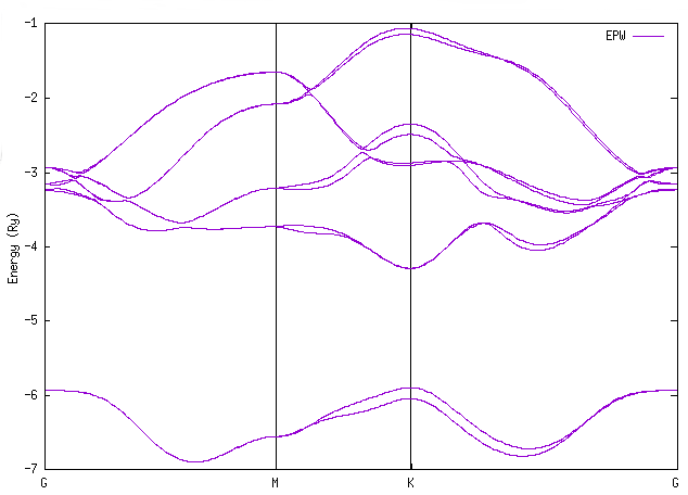
We can also compare the phonon bandstructures:

$ gnuplot
gnuplot> set terminal x11 enhanced
gnuplot> set encoding utf8
gnuplot> set ylabel "{/Symbol w} (meV)"
gnuplot> set xtics ("{/Symbol G}" 0, "M" 0.5774, "K" 0.9157, "{/Symbol G}" 1.5773)
gnuplot> set arrow from 0.5774, graph 0 to 0.5774, graph 1 nohead
gnuplot> set arrow from 0.9107, graph 0 to 0.9107, graph 1 nohead
gnuplot> plot "freq.dat" u 1:2 w l title "EPW"

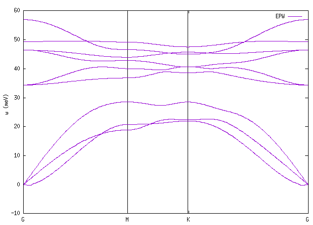
where you can notice the small imaginary phonon close to $\Gamma$ due to unconverged results. Interestingly, you can zoom on the LO and TO modes around 45 meV. In 2D they are degenerate at q=$\Gamma$ but with a linear slope discontinuity.

At convergence you should get a phonon dispersion similar to this where DD means dipole-dipole, DQ means dipole-quadrupole and QQ means quadrupole-quadrupole interaction [3]: .. image:: figures/MoS2-phonon.pdf

alt:

Tutorial result

align:

center

class:

tutorial-figure tutorial-large

Action: Perform an restart calculation to obtain the electron-phonon matrix element at k=$\Gamma$ and for q along the same high-symmetry path:

epw2.in

&inputepw
  prefix      = 'mos2'
  outdir      = './'

  elph        = .true.
  epbwrite    = .false.
  epbread     = .false.
  epwwrite    = .false.
  epwread     = .true.

  etf_mem     = 1
  lpolar      = .true.
  vme         = 'wannier'

  use_ws      = .true.
  lifc        = .false.

  nbndsub     =  10
  bands_skipped = 'exclude_bands = 1-24'

  system_2d   = 'quadrupole'

  wannierize  = .false.
  num_iter    = 5000
  iprint      = 2
  dis_win_max = -0.8
  dis_win_min = -6.8
  dis_froz_max= -3.6
  proj(1)     = 'Mo:d'
  wdata(1) = 'bands_plot = .true.'
  wdata(2) = 'begin kpoint_path'
  wdata(3) = 'G 0.00 0.00 0.00 M 0.50 0.00 0.00'
  wdata(4) = 'M 0.50 0.00 0.00 K 0.333333333333 0.333333333333 0.00'
  wdata(5) = 'K 0.333333333333 0.333333333333 0.00 G 0.0 0.0 0.00'
  wdata(6) = 'end kpoint_path'
  wdata(7) = 'bands_plot_format = gnuplot'
  wdata(8) = 'dis_num_iter      = 5000'
  wdata(9) = 'num_print_cycles  = 10'
  wdata(10) = 'dis_mix_ratio     = 1.0'
  wdata(11) = 'conv_tol = 1E-12'
  wdata(12) = 'conv_window = 4'

  fsthick     = 20 ! eV
  nstemp      = 1
  temps       = 300
  degaussw    = 0.01 ! eV

  dvscf_dir   = './save'

  prtgkk      = .true.

  nkf1         = 1
  nkf2         = 1
  nkf3         = 1
  filqf        = './GMKG.txt'

  nk1         = 6
  nk2         = 6
  nk3         = 1
  nq1         = 6
  nq2         = 6
  nq3         = 1
 /

$ ibrun -n 56 $PATHQE/bin/epw.x -in epw2.in -nk 56 1> epw2.out 2> error.out

We will not analyze the result in detail here but take a look at the output. You can compare interpolated matrix elements with the one obtained by direct calculation to assess the quality of the interpolation.

Action: Perform an restart calculation to obtain the electron drift and Hall mobility on an interpolated 30$\times$30$\times$1 fine k-point and q-point grids.

We suggest working in a different directory for each restart calculations to avoid potential data conflict. For this, you can move in the restart folder and perform a soft link of all the required file for a restart:

$ cd restart
ln -s ../crystal.fmt
ln -s ../epwdata.fmt
ln -s ../mos2.bvec
ln -s ../mos2.chk
ln -s ../mos2.kgmap
ln -s ../mos2.mmn
ln -s ../mos2.nnkp
ln -s ../mos2.ukk
ln -s ../mos2.epmatwp
ln -s ../vmedata.fmt
ln -s ../save
ln -s ../quadrupole.fmt
ln -s ../dmedata.fmt

$ ibrun -n 56 $PATHQE/bin/epw.x -in epw3.in -nk 56 1> epw3.out 2> error.out

epw3.in

&inputepw
  prefix      = 'mos2'
  outdir      = './'

  elph        = .true.
  epbwrite    = .false.
  epbread     = .false.
  epwwrite    = .false.
  epwread     = .true.

  etf_mem     = 3
  mp_mesh_k   = .true.
  lpolar      = .true.
  vme         = 'wannier'

  use_ws      = .true.
  lifc        = .false.

  nbndsub     =  10
  bands_skipped = 'exclude_bands = 1-24'

  system_2d   = 'quadrupole'

  scattering  = .true.
  scattering_serta = .true.
  int_mob     = .false.
  carrier     = .true.
  ncarrier    =  1E10
  iterative_bte = .true.
  epmatkqread = .false.
  mob_maxiter = 100
  broyden_beta= 1.0
  bfieldx     = 0.0d0
  bfieldy     = 0.0d0
  bfieldz     = 1.0d-10

  nstemp      = 2
  temps       = 300 500

  restart      = .true.
  selecqread   = .false.

  wannierize  = .false.
  num_iter    = 5000
  iprint      = 2
  dis_win_max = -0.8
  dis_win_min = -6.8
  dis_froz_max= -3.6
  proj(1)     = 'Mo:d'
  wdata(1) = 'bands_plot = .true.'
  wdata(2) = 'begin kpoint_path'
  wdata(3) = 'G 0.00 0.00 0.00 M 0.50 0.00 0.00'
  wdata(4) = 'M 0.50 0.00 0.00 K 0.333333333333 0.333333333333 0.00'
  wdata(5) = 'K 0.333333333333 0.333333333333 0.00 G 0.0 0.0 0.00'
  wdata(6) = 'end kpoint_path'
  wdata(7) = 'bands_plot_format = gnuplot'
  wdata(8) = 'dis_num_iter      = 5000'
  wdata(9) = 'num_print_cycles  = 10'
  wdata(10) = 'dis_mix_ratio     = 1.0'
  wdata(11) = 'conv_tol = 1E-12'
  wdata(12) = 'conv_window = 4'

  degaussw    = 0.01
  dvscf_dir   = './save'

  fsthick      = 0.4  ! eV
  efermi_read  = .true
  fermi_energy = -4.391448 ! CBM = -4.291448

  nkf1         = 60
  nkf2         = 60
  nkf3         = 1
  nqf1         = 60
  nqf2         = 60
  nqf3         = 1

  nk1         = 6
  nk2         = 6
  nk3         = 1
  nq1         = 6
  nq2         = 6
  nq3         = 1
 /

Note 1: etf_mem = 3 is an important input to reduce computational cost by considering momentum within the thickness window.
Note 2: ncarrier = 1E10 indicates the electron mobility calculation with a concentration of 1E10 cm\(^{-2}\).
Note 3: degaussw = 0.01 means we are using gaussian smearing.
Note 4: The Fermi energy is chosen 0.1 eV below the CBM. The value of the CBM can be found in the output:

Valence band maximum    =  -5.893225 eV
Conduction band minimum =  -4.291448 eV

At the end, you should obtain a 134 cm$^2$/Vs room temperature SERTA and 129 cm$^2$/Vs IBTE drift mobility. The associated Hall factor is also reported.

Action: Perform an restart calculation to obtain the hole drift and Hall mobility on an interpolated 30$\times$30$\times$1 fine $\bf{k}$-point and $\bf{q}$-point grids.

$ rm restart_0.fmt
$ ibrun -n 56 $PATHQE/bin/epw.x -in epw4.in -nk 56 1> epw4.out 2> error.out

epw4.in

&inputepw
  prefix      = 'mos2'
  outdir      = './'

  elph        = .true.
  epbwrite    = .false.
  epbread     = .false.
  epwwrite    = .false.
  epwread     = .true.

  etf_mem     = 3
  mp_mesh_k   = .true.
  lpolar      = .true.
  vme         = 'wannier'

  use_ws      = .true.
  lifc        = .false.

  nbndsub     =  10
  bands_skipped = 'exclude_bands = 1-24'

  system_2d   = 'quadrupole'

  scattering  = .true.
  scattering_serta = .true.
  int_mob     = .false.
  carrier     = .true.
  ncarrier    =  -1E10
  iterative_bte = .true.
  epmatkqread = .false.
  mob_maxiter = 100
  broyden_beta= 1.0
  bfieldx     = 0.0d0
  bfieldy     = 0.0d0
  bfieldz     = 1.0d-10

  nstemp      = 2
  temps       = 300 500

  restart      = .true.
  selecqread   = .false.

  wannierize  = .false.
  num_iter    = 5000
  iprint      = 2
  dis_win_max = -0.8
  dis_win_min = -6.8
  dis_froz_max= -3.6
  proj(1)     = 'Mo:d'
  wdata(1) = 'bands_plot = .true.'
  wdata(2) = 'begin kpoint_path'
  wdata(3) = 'G 0.00 0.00 0.00 M 0.50 0.00 0.00'
  wdata(4) = 'M 0.50 0.00 0.00 K 0.333333333333 0.333333333333 0.00'
  wdata(5) = 'K 0.333333333333 0.333333333333 0.00 G 0.0 0.0 0.00'
  wdata(6) = 'end kpoint_path'
  wdata(7) = 'bands_plot_format = gnuplot'
  wdata(8) = 'dis_num_iter      = 5000'
  wdata(9) = 'num_print_cycles  = 10'
  wdata(10) = 'dis_mix_ratio     = 1.0'
  wdata(11) = 'conv_tol = 1E-12'
  wdata(12) = 'conv_window = 4'

  degaussw    = 0.0
  dvscf_dir   = './save'

  fsthick      = 0.4  ! eV
  efermi_read  = .true
  fermi_energy = -5.793225 ! VBM = -5.893225

  nkf1         = 60
  nkf2         = 60
  nkf3         = 1
  nqf1         = 60
  nqf2         = 60
  nqf3         = 1

  nk1         = 6
  nk2         = 6
  nk3         = 1
  nq1         = 6
  nq2         = 6
  nq3         = 1
 /

where here you should obtain a room temperature hole drift SERTA and IBTE mobility of 33 cm$^2$/Vs and 35 cm$^2$/Vs, respectively. However here the Hall factor is quite big.

At convergence you should get a temperature dependent Hall mobility and Hall factor similar to this [4]: .. image:: figures/mos2-mob.pdf

alt:

Tutorial result

align:

center

class:

tutorial-figure tutorial-default

Exercise 3¶

In this example we are going to calculate the electrical resistivity of bcc Fe using the BTE. Fe is a ferromagnetic metal and we will consider 2 cases. A non-magnetic calculation and a collinear magnetic calculation. In the non magnetic case EPW calculates the conductivity as:

\[\sigma_{\alpha\beta} = \frac{-e}{V_{\mathrm{uc}}} \sum_n \! \int \! \frac{\mathrm{d}^3 k}{\Omega_{\mathrm{BZ}}} \, v_{n\mathbf{k}\alpha} \partial_{E_{\beta}} f_{n\mathbf{k}}\]

First go in the third exercise:

$ cd exercise3

3.1 Conductivity in a non-magnetic compound¶

You will find two folders. One for the non-magnetic calculation, and another one for the ferromagnetic case. Lets start with the non magnetic case:

$ cd NM

Action: Make a self-consistent calculation for Fe and a phonon calculation on a homogeneous 3x3x3 $\bf{q}$-point grid.

Note: The ecutwfc and $\mathbf{k}$-mesh grid needs to be larger for real calculations.

$ ibrun -n 56 $PATHQE/bin/pw.x -in scf.in -nk 8 1> scf.out 2> error.out
$ ibrun -n 56 $PATHQE/bin/ph.x -in ph.in -nk 8 1> ph.out 2> error.out

scf.in

&CONTROL
 outdir='./'
 calculation='scf',
 restart_mode='from_scratch',
 prefix='fe',
 pseudo_dir = '../../pseudo/'
/

&SYSTEM
 ibrav=3,
 celldm(1)=5.0929838463,
 nat=1,
 ntyp=1,
 nspin = 2,
 starting_magnetization(1)=2,
 ecutwfc=60.0,
 occupations='smearing',
 smearing='mv',
 degauss=0.025,
/
&ELECTRONS
mixing_beta=0.7,
conv_thr=1d-8,
/
ATOMIC_SPECIES
Fe 55.8457 Fe.pz.upf
ATOMIC_POSITIONS (alat)
Fe 0 0 0
K_POINTS automatic
8 8 8 0 0 0

ph.in

&inputph
  tr2_ph=1.0d-16,
  prefix='fe',
  amass(1)=55.8457,
  outdir='./',
  fildyn='fe.dyn.xml',
  fildvscf='dvscf'
  ldisp=.true.,
  nq1 = 3,
  nq2 = 3,
  nq3 = 3
/

The important keyword is fildvscf as it will tell the code to write to file the change of potential due to ionic displacement $\partial_{\mathbf{q}\nu}V^\mathrm{scf}$. The ldisp input allows to calculate phonons for a grid of $\mathbf{q}$-points specified by nq1, nq2, and nq3.

Note 1: For real calculations in metals, the coarse \(\mathbf{q}\)-point and \(\mathbf{k}\)-point grids should be converged on and are typically 6\(\times\)6\(\times\)6 or 8\(\times\)8\(\times\)8 and 18\(\times\)18\(\times\)18 or 24\(\times\)24\(\times\)24 respectively.
Note 2: The tr2_ph variable is the threshold on the perturbed wavefunction obtained by solving the Sternheimer equation and should be very small.
Note 3: It is recommended to add XXX.xml at the end of the fildyn as it will force the code to write the output in XML format.

This calculation should take about 5 min to be completed. In the output file, locate the list of 4 irreducible q points in the Brillouin Zone (IBZ):

Dynamical matrices for ( 3, 3, 3)  uniform grid of q-points
(   4 q-points):
  N         xq(1)         xq(2)         xq(3)
  1   0.000000000   0.000000000   0.000000000
  2   0.000000000  -0.333333333   0.333333333
  3  -0.333333333   0.666666667  -0.333333333
  4   0.000000000   0.000000000   0.666666667

For each q-point, a fe.dynX.xml file containing the dynamical matrix has been produced. The pb.dvscf files are located inside the _ph0 folder.

Action: Gather the .dynX.xml, .dvscf and patterns [5] files into a new save directory. This can easily be done using the pp.py python script.

$ python3 $PATHQE/EPW/bin/pp.py

The script will ask you to provide the prefix of your calculation (here “fe”).

Action: Do a non self-consistent calculation on a homogeneous 3$\times$3$\times$3 uniform and :math:`Gamma`-centered grid in the interval [0,1) in crystal coordinates.

$ ibrun -n 56 $PATHQE/bin/pw.x -in nscf.in -nk 8 1> nscf.out 2> error.out

nscf.in

&CONTROL
 outdir='./'
 calculation='bands',
 prefix='fe',
 pseudo_dir = '../../pseudo/'
/

&SYSTEM
 ibrav=3,
 celldm(1)=5.0929838463,
 nat=1,
 ntyp=1,
 ecutwfc=60.0,
 occupations='smearing',
 smearing='mv',
 degauss=0.025,
/
&ELECTRONS
mixing_beta=0.7,
conv_thr=1d-8,
/
ATOMIC_SPECIES
Fe 55.8457 Fe.pz.upf
ATOMIC_POSITIONS (alat)
Fe 0 0 0
K_POINTS crystal
27
  0.00000000  0.00000000  0.00000000  3.703704e-02
  0.00000000  0.00000000  0.33333333  3.703704e-02
  0.00000000  0.00000000  0.66666667  3.703704e-02
  0.00000000  0.33333333  0.00000000  3.703704e-02
...

Note : The $\mathbf{k}$-point grid from nscf.in and the $\mathbf{q}$-point grid from ph.in have to be commensurate with each other. The $\mathbf{k}$-point grid in scf.in can be arbitrary.

$ ibrun -n 56 $PATHQE/bin/pw.x -input nscf.in -npool 8 1> nscf.out 2> error.out

Action: Prepare the EPW input file. Here we will interpolate the matrix elements from a coarse 3$\times$3$\times$3 to a dense 30$\times$30$\times$30 $\mathbf{k}$-point and $\mathbf{q}$-point grids. Then we compute the conductivity of non magnetic Fe using the BTE.

$ ibrun -n 56 $PATHQE/bin/epw.x -in epw1.in -nk 56 1> epw1.out 2> error.out

epw1.in

&inputepw
  prefix = 'fe',
  amass(1) = 55.8457
  dvscf_dir = 'save'
  etf_mem = 1

  elph = .true.
  epwwrite = .true.
  epwread = .false.

  wannierize = .true.
  bands_skipped = 'exclude_bands = 1-4'
  nbndsub = 9
  num_iter = 800
  dis_win_max = 65
  dis_froz_max= 35
  proj(1) = 'Fe:sp3d2'
  proj(2) = 'Fe:dxz,dyz,dxy'
  use_ws = .false.
  wdata(1) = 'bands_plot = .true.'
  wdata(2) = 'begin kpoint_path'
  wdata(3) = 'G 0.000  0.000  0.000 H 0.500 -0.500 -0.500'
  wdata(4) = 'H 0.500 -0.500 -0.500 P 0.750  0.250 -0.250'
  wdata(5) = 'P 0.750  0.250 -0.250 G 0.000  0.000  0.000'
  wdata(6) = 'G 0.000  0.000  0.000 N 0.000  0.000 -0.500'
  wdata(7) = 'end kpoint_path'
  wdata(9) = 'bands_num_points = 50'
  wdata(10) = 'dis_num_iter = 800'
  wdata(11) = 'num_print_cycles = 10'
  wdata(12) = 'conv_tol = 1E-12'
  wdata(13) = 'conv_window = 4'
  wdata(14) = 'bands_plot_format = gnuplot'

  fsthick = 0.3
  degaussw = 0.005
  assume_metal = .true.
  ngaussw = -99

  int_mob = .false.
  iterative_bte = .true.
  scattering = .true.
  carrier = .false.
  mp_mesh_k = .true.
  epmatkqread = .false
  mob_maxiter = 200
  restart_step = 100
  selecqread = .false.
  nstemp = 2
  temps = 200 300

  nkf1 = 30
  nkf2 = 30
  nkf3 = 30
  nqf1 = 30
  nqf2 = 30
  nqf3 = 30

  nq1 = 3
  nq2 = 3
  nq3 = 3
  nk1 = 3
  nk2 = 3
  nk3 = 3
/

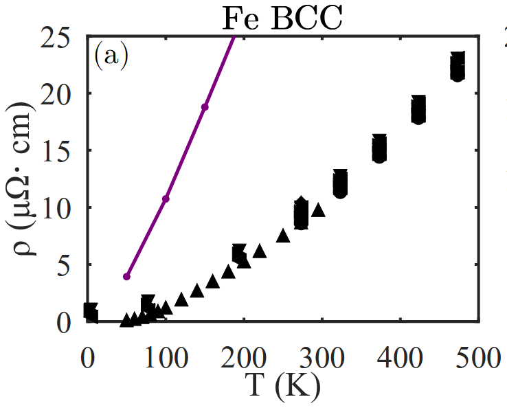
Note 1: Tha main difference with the input for mobility are assume_metal = .true. and carrier = .false.
Note 2: Here we are both wannierizing, unfolding, interpolating matrix elements and computing the resistivity. In practice, the typical workflow is in two steps. First, verify that the interpolation is correct. Second, compute the resistivity until convergence
Note 3: For a two step procedure we would typically first set epwwrite = .true. and epwread = .true. with bands_plot = .true. to verify the band interpolation and prtgkk = .true. for the matrix element interpolation. Then we would do a restart calculation with epwwrite = .false. and epwread = .true. and all the BTE related input flags.
Note 4: Here we use a fixed smearing degaussw = XXX. If degaussw = 0.0 we use adaptative smearing, we recommend to use a fixed but small smearing  [6].
Note 5: The fsthick determines the volume around the Fermi surface that would contribute to transport. This value changes with temperature. We recommend either providing the one with the highest temperature or carefully tuning it. Typical values should be around 0.25-0.5 eV.

Action: Extract the conductivity values for different temperatures and try to make a plot. Action: Increase the temperature to get more data points. | However, if we compare with the experiments, we are overestimating the resistivity. The main reason is that the phonons are unstable in bcc Fe when we use the non magnetic approximation and as a result the matrix elements $g_{mn\nu}(\mathbf{k},\mathbf{q})\propto \omega_{\mathbf{q}\nu}^{-\frac{1}{2}}$ would be overestimated [7]:

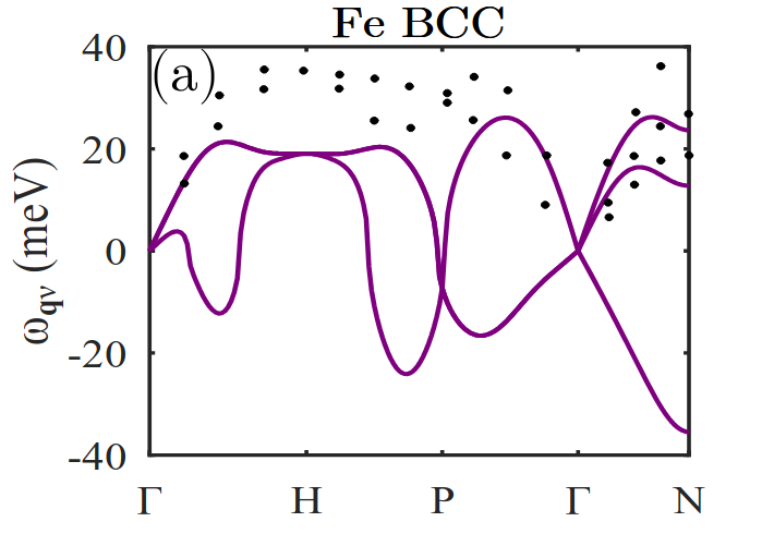
We can verify this with q2r.x and matdyn.x

$ $PATHQE/bin/q2r.x < q2r.in | tee q2r.out
$ $PATHQE/bin/matdyn.x < matdyn.in | tee matdyn.out

q2r.in

&input
 fildyn='fe.dyn.xml',
 zasr='crystal',
 flfrc='fe.fc',
/

matdyn.in

&input
 asr='crystal',
 amass(1)=55.845,
 flfrc='fe.fc.xml',
 flfrq='fe.freq',
 flvec='fe.modes'
 q_in_band_form = .true.
 q_in_cryst_coord = .false.
/
5
0.000000     0.000000     0.000000 50 ! G
0.000000     1.000000     0.000000 50 ! H
0.500000     0.500000     0.500000 50 ! P
0.000000     0.000000     0.000000 50 ! G
0.500000     0.500000     0.000000 50 ! N

3.2 Conductivity in a magnetic compound¶

We now repeat the procedure but in this case using the ferromagnetic calculation at collinear level.

$ cd ../FM

Action: Make a self-consistent calculation for ferromagnetic Fe and a phonon calculation on a homogeneous 3x3x3 $\bf{q}$-point grid.

scf.in

&CONTROL
 outdir='./'
 calculation='scf',
 prefix='fe',
 pseudo_dir = '../../pseudo/'
/

&SYSTEM
 ibrav=3,
 celldm(1)=5.201879033248,
 nat=1,
 ntyp=1,
 nspin = 2,
 starting_magnetization(1)=2.0,
 ecutwfc=60.0,
 occupations='smearing',
 smearing='mv',
 degauss=0.025,
/
&ELECTRONS
  mixing_beta=0.7,
  conv_thr=1d-8,
/
ATOMIC_SPECIES
  Fe 55.8457 Fe.pz.upf
ATOMIC_POSITIONS (alat)
  Fe 0 0 0
K_POINTS automatic
8 8 8 0 0 0

ph.in

&inputph
  tr2_ph=1.0d-16,
  prefix='fe',
  amass(1)=55.8457,
  outdir='./',
  fildyn='fe.dyn.xml',
  fildvscf='dvscf'
  ldisp=.true.,
  nq1 = 3,
  nq2 = 3,
  nq3 = 3
/

Note

For collinear magnetism we need the input flags nspin = 2 and starting_magnetization(1) = XX.X to non zero value to set the magnetization of a given atomic species in the scf.in. In the case of insulators we would also need to provide tot_magnetization = XX.X to fix the total magnetization.
The scf.in has different cell parameter celldm(1)=5.201879 than those in the non magnetic case. Each magnetic configuration needs its own cell parameters. In practice, one needs to relax for each magnetic order.

For each $\bf{q}$-point, a fe.dynX.xml file containing the dynamical matrix has been produced. The fe.dvscf files are located inside the _ph0 folder.

Action: Gather the .dynX.xml, .dvscf and patterns [8] files into a new save directory. This can easily be done using the pp.py python script.

$ python3 $PATHQE/EPW/bin/pp.py

We can now verify that the phonons are stable in the ferromagnetic case, the q2r.in and matdyn.in inputs are the same as in the non magnetic case

$ $PATHQE/bin/q2r.x < q2r.in | tee q2r.out
$ $PATHQE/bin/matdyn.x < matdyn.in | tee matdyn.out

As you can see the phonons are now stable [9]. Consequently, it is obvious that for magnetic systems it is crucial to include the spin degree of freedom in the calculations, even if its just at collinear level.

Action: Make a non self-consistent calculation

$ ibrun -n 56 $PATHQE/bin/pw.x -in nscf.in -nk 8 1> nscf.out 2> error.out

nscf.in

&CONTROL
 outdir='./'
 calculation='bands',
 prefix='fe',
 pseudo_dir = '../../pseudo/'
/

&SYSTEM
 ibrav=3,
 celldm(1)=5.201879033248,
 nat=1,
 ntyp=1,
 nspin = 2,
 starting_magnetization(1)=2,
 ecutwfc=60.0,
 occupations='smearing',
 smearing='mv',
 degauss=0.025,
/
&ELECTRONS
  mixing_beta=0.7,
  conv_thr=1d-8,
/
ATOMIC_SPECIES
  Fe 55.8457 Fe.pz.upf
ATOMIC_POSITIONS (alat)
  Fe 0 0 0
K_POINTS crystal
27
  0.00000000  0.00000000  0.00000000  3.703704e-02
  0.00000000  0.00000000  0.33333333  3.703704e-02
  0.00000000  0.00000000  0.66666667  3.703704e-02
  0.00000000  0.33333333  0.00000000  3.703704e-02
...

Action: Create two separate folders: one for spin up and another one for spin down. We need to link the fe.save and the save folders inside here

$ mkdir up dn
$ cd up
$ ln -s ../fe.save
$ ln -s ../save
$ cd ../dn
$ ln -s ../fe.save
$ ln -s ../save
$ cd ../

The local spin density approximation (LSDA) option in EPW requires to first perform the unfolding and wannierizing procedure of the two spin channels first without interpolating. Then one can compute any interpolated property.

Action: Copy the epw1_lsda.in input file to each of the two folders.

$ cp epw1_lsda.in up
$ cp epw1_lsda.in dn

epw1_lsda.in

&inputepw
  prefix = 'fe',
  amass(1) = 55.8457
  dvscf_dir = 'save'
  etf_mem = 1

  elph = .true.
  epwwrite = .true.
  epwread = .false.

  interpolate = .false.
  lsda = 'up' ! 'up' or 'down' depending on each spin channel

  wannierize = .true.
  bands_skipped = 'exclude_bands = 1-4'
  nbndsub = 9
  num_iter = 500
  dis_win_max = 60
  dis_froz_max= 30
  proj(1) = 'Fe:sp3d2'
  proj(2) = 'Fe:dxz,dyz,dxy'
  use_ws = .false.
  wdata(1) = 'bands_plot = .true.'
  wdata(2) = 'begin kpoint_path'
  wdata(3) = 'G 0.000  0.000  0.000 H 0.500 -0.500 -0.500'
  wdata(4) = 'H 0.500 -0.500 -0.500 P 0.750  0.250 -0.250'
  wdata(5) = 'P 0.750  0.250 -0.250 G 0.000  0.000  0.000'
  wdata(6) = 'G 0.000  0.000  0.000 N 0.000  0.000 -0.500'
  wdata(7) = 'end kpoint_path'
  wdata(9) = 'bands_num_points = 50'
  wdata(10) = 'dis_num_iter = 800'
  wdata(11) = 'num_print_cycles = 10'
  wdata(12) = 'conv_tol = 1E-12'
  wdata(13) = 'conv_window = 4'
  wdata(14) = 'bands_plot_format = gnuplot'

  nkf1 = 1
  nkf2 = 1
  nkf3 = 1
  nqf1 = 1
  nqf2 = 1
  nqf3 = 1

  nq1 = 3
  nq2 = 3
  nq3 = 3
  nk1 = 3
  nk2 = 3
  nk3 = 3
/

Action: Edit the input files setting the input flag lsda = ’up’ or lsda = ’down’ to set the spin channel. | Notes:

In EPW we activate the LSDA module by providing the input flag lsda = ’up’ or lsda = ’down’. The default is non magnetic lsda = ’none’
In the LSDA workflow, we need first to unfold the two spin channels before interpolating. This is controlled with the input flag interpolate = .false.. The default is interpolate = .true.
The input flag interpolate is not exclusive to the LSDA module. It can be used in non magnetic case to just wannierize and made the unfolding procedure. This is useful if one just needs EPW to interface with other codes.
In the unfolding procedure we set epwwrite = .true. and epwread = .false.
The LSDA module is currently tested with both LDA and GGA type of density functionals.

Action: Run EPW and unfold both spin channels.

$ cd up
$ ibrun -n 56 $PATHQE/bin/epw.x -in epw1_lsda.in -nk 56 1> epw1.out 2> error.out
$ cd ../dn
$ ibrun -n 56 $PATHQE/bin/epw.x -in epw1_lsda.in -nk 56 1> epw1.out 2> error.out

This calculation should have generated several .fmt files and the .epmatwp files. In the case of lsda = ’down’ you would notice that the files contain the string .down in their name, i.e.XXX.down.XXX.

Action: Link the .fmt files that contain the name crystal, epwdata or wigner of the opposite spin channel.

$ cd up
 ln -s ../dn/crystal.down.fmt
 ln -s ../dn/epwdata.down.fmt
 ln -s ../dn/wigner.down.fmt
$ cd ../dn
 ln -s ../up/crystal.fmt
 ln -s ../up/epwdata.fmt
 ln -s ../up/wigner.fmt

We are now ready to use EPW and interpolate the quantity that we are interested in. In this tutorial we are interested in the resistivity of ferromagnetic Fe. In particular, EPW computes the spin resolved conductivity

\[\begin{aligned} \sigma^{\mathrm{\sigma}}_{\alpha\beta} = \frac{-e}{V^{\mathrm{uc}}} \sum_n \! \int \! \frac{\mathrm{d}^3 k}{\Omega^{\mathrm{BZ}}} \, v^\sigma_{n\mathbf{k}\alpha} \partial_{E_{\beta}} f^\sigma_{n\mathbf{k}}, \end{aligned}\]

for a given spin channel $\sigma = \{\uparrow,\downarrow\}$. To compute the total resistivity $\rho_{\alpha\beta}$, we extract the spin resolved conductivity and we use the following formula

(6)¶\[ \begin{align}\begin{aligned}\begin{aligned} \rho_{\alpha\beta} = (\sigma^\uparrow_{\alpha\beta}+\sigma^\downarrow_{\alpha\beta})^{-1}.\\\end{aligned}\end{aligned}\end{align} \]

Action: Copy the epw2_lsda.in input file to each folder up or dn and modify the lsda input flag accordingly lsda = ’up’ or lsda = ’down’.

$ cp epw2_lsda.in up
$ cp epw2_lsda.in dn

Action: Run EPW to compute the spin resolved conductivity with the BTE for each spin channel.

$ cd up
$ ibrun -n 56 $PATHQE/bin/epw.x -in epw2_lsda.in -nk 56 1> epw2.out 2> error.out
$ cd ../dn
$ ibrun -n 56 $PATHQE/bin/epw.x -in epw2_lsda.in -nk 56 1> epw2.out 2> error.out

epw2_lsda.in

&inputepw
  prefix = 'fe',
  amass(1) = 55.8457
  dvscf_dir = 'save'
  etf_mem = 1

  elph = .true.
  epwwrite = .false.
  epwread = .true.

  wannierize = .false.
  bands_skipped = 'exclude_bands = 1-4'
  nbndsub = 9
  use_ws = .false.

  fsthick = 0.3
  degaussw = 0.005
  assume_metal = .true.
  ngaussw = -99

  int_mob = .false.
  iterative_bte = .true.
  scattering = .true.
  carrier = .false.
  mp_mesh_k = .true.
  epmatkqread = .false
  mob_maxiter = 200
  restart_step = 100
  selecqread = .false.
  nstemp = 9
  temps = 100 500

  nkf1 = 30
  nkf2 = 30
  nkf3 = 30
  nqf1 = 30
  nqf2 = 30
  nqf3 = 30

  nq1 = 3
  nq2 = 3
  nq3 = 3
  nk1 = 3
  nk2 = 3
  nk3 = 3
/

Note 1: In this calculation, we are restarting from the electron-phonon matrix elements written in real space in the fe.epmatwp or fe.down.epmatwp files.
Note 2: In the case of BTE, temps corresponds to the real lattice temperature and degaussw is used to approximate the Dirac deltas. In this case we take a small smearing value 0.005 eV in a similar spirit as the smearing in the scf.in.
Note 3: Because of the restart = .true. input parameter, if you want to do a clean restart, you need to remove the restart file by doing rm restart_0.fmt or rm restart.down_0.fmt.

Action: Extract the SERTA and BTE conductivity as a function of temperature from the output file. You should obtain something like: .. image:: figures/Fe-cond.png

alt:

Tutorial result

align:

center

class:

tutorial-figure tutorial-default

Action: Use Eq. (6) to compute the resistivity, at convergence you should get [10]: .. image:: figures/Fe-res-EPW-school.pdf

alt:

Tutorial result

align:

center

class:

tutorial-figure tutorial-default

Action: You can try changing the pseudo from LDA to GGA and see the effect on the resistivity. Action: Check the difference between SERTA and BTE. Usually in metals is not very pronouced | Notes:

In magnetic systems apart from electron-phonon scattering we would also have electron-magnon scattering which we neglect here, see arXiv:2501.11350 (2025). Hence we generally underestimate the resistivity
Using the LSDA module for mobility instead of resistivity is also possible using the same workflow and modifying the inputs accordingly. In the case of the mobility it is advised to provide an extra input gap_energy such that $\varepsilon_\mathrm{VBM} <$ gap_energy $< \varepsilon_\mathrm{CBM}$ in the case of wannierizing both part of the valence and conduction band manifolds
For semiconductors EPW computes the spin resolved mobility $\mu^\sigma_{\alpha\beta}\equiv\frac{\sigma^\sigma_{\alpha\beta}}{n^\sigma_\mathrm{c}}$. The total mobility should be computed as $\mu^\mathrm{eff}_{\alpha\beta} = \frac{n^\uparrow_{\mathrm{c}} \mu^\uparrow_{\alpha\beta}+n^\downarrow_{\mathrm{c}}\mu^\downarrow_{\alpha\beta}}{n^\uparrow_\mathrm{c}+n^\downarrow_\mathrm{c}}$, with $n^\sigma_\mathrm{c}$ the carrier concentration on the spin channel $\sigma$. In practice one should use the same value for ncarrier which is the total carrier concentration.
Not all EPW modules are compatible with LSDA yet.
Compatible modules with LSDA beyond transport are spectral functions using the flags a2f = .true., phonselfen = .true. and elecselfen = .true. which can be used to calculate spin resolved $\Pi^\sigma_{\mathbf{q}\nu}$, $\lambda^\sigma_{\mathbf{q}\nu}$ and $\Sigma^\sigma_{n\mathbf{k}}$.
The LSDA module is compatible with 2D systems as well. In this case it might be useful to set use_ws = .true. specially for insulators.

T (K)	hole \(\varepsilon_F\) (eV)	drift SERTA \(\mu\) (cm\(^2\)/Vs)	drift BTE \(\mu\) (cm\(^2\)/Vs)	Hall BTE \(\mu\) (cm\(^2\)/Vs)
100
200
300
400
500