Exciton polarons and self-trapped excitons
This tutorial is in draft state and is currently being updated
09/15/2026
Note
Hands-on based on Quantum ESPRESSO v7.6, EPW v6.1, and BerkeleyGW v4.0.
Introduction
In this tutorial, we will show how to compute exciton polarons in lithium fluoride (LiF) using the ab initio exciton polaron equations that are published in Phys. Rev. Lett. 132, 036902 (2024) and Phys. Rev. B 109, 045202 (2024):
where \(E_{s\mathbf{Q}}^0\) are the Bethe-Salpeter equation (BSE) eigenvalues of the undistorted structure, and \(\mathcal{G}_{ss'\nu}( \mathbf{Q}, \mathbf{q})\) denote exciton-phonon coupling matrix elements:
Here, \(a_{vc\mathbf{k}}^{s\mathbf{Q}}\) are the finite-momentum BSE eigenvectors under the Tamm-Dancoff approximation:
and \(g_{mn\nu}(\mathbf{k},\mathbf{q})\) are the usual electron-phonon coupling matrix elements:
We are going to use Quantum ESPRESSO and EPW to calculate the phonon vibrational frequencies \(\omega_{\mathbf{q}\nu}\) and eigenmodes \(e_{\kappa\alpha,\nu}(\mathbf{q})\), as well as the electron-phonon coupling matrix elements \(g_{mn\nu}(\mathbf{k},\mathbf{q})\). Meanwhile, the BSE eigenvalues and eigenvectors are obtained using BerkeleyGW.
Important: The Kohn-Sham wave functions appearing in Eq. (3) and Eq. (4) must be exactly the same. Otherwise, the calculated results are incorrect and unpredictable.
The calculations consist of 5 major steps:
DFT calculations to obtain the converged charge density. Kohn-Sham wave functions on a uniform Brillouin-zone grid without symmetry reduction are also obtained in this step.
GW calculations to obtain the dielectric functions and the corrected electronic band structures.
BSE calculations to obtain the exciton eigenvalues and eigenvectors with finite momentum on a uniform Brillouin-zone grid.
DFPT calculations to obtain the phonon vibrational frequencies and eigenvectors, as well as the variation of the Kohn-Sham potentials.
EPW calculations to construct the exciton-phonon coupling matrix elements and solve the ab initio exciton polaron equations.
The files that are needed for these calculations can be accessed in your cluster (Frontera@TACC for most people) through:
wget --content-disposition \
"https://drive.google.com/uc?export=download&id=1CywB3rCe4RVeMLLea3lOy7rlqwgPvbAZ"
tar xvf Sat.5.Dai.tar
cd Sat.5.Dai/
Preliminaries (optional)
Note: To finish this tutorial, please skip this section and use the provided executables stored in /work2/05193/sabyadk/shared/EPW_6.1s/q-e/bin. If you want to build Quantum ESPRESSO/EPW yourself with HDF5 support later in your own computing environment, consult the steps outlined in the rest of this section.
To calculate exciton polarons in practice, you will need to compile Quantum ESPRESSO/EPW and BerkeleyGW with the HDF5 support. This is to make sure that the BSE eigenvectors generated by BerkeleyGW can be correctly read by EPW.
To enable the HDF5 support of Quantum ESPRESSO, we use the supercomputer Frontera at TACC as an example. Execute the following command in the terminal of Frontera:
module load hdf5
Then, go to the directory of the Quantum ESPRESSO source code, and configure your QE installation with HDF5 support:
cd YOUR/QE/PATH
./configure --with-hdf5=${TACC_HDF5_DIR}
make -j4 epw
To compile BerkeleyGW with HDF5 support, please consult the instructions provided in the BerkeleyGW source codes.
DFT calculations
This whole step can be finished by submitting the jobscript run.espresso.sh
sbatch run.espresso.sh
which contains the following:
#!/bin/bash
#SBATCH -J lif                 # Job name
#SBATCH -p normal              # Queue (partition) name
#SBATCH -N 1                   # Total # of nodes
#SBATCH -n 56                  # Total # of mpi tasks
#SBATCH -t 00:30:00            # Run time (hh:mm:ss)
#SBATCH -A DMR23048            # Project/Allocation name (req'd if you have more than 1)
#SBATCH --reservation=MATCSSI_Norm_June20

# Load modules required for QE
module load hdf5/1.10.4

bash espresso/link.sh
cd espresso/01-Density
bash run.sh
cd ../..

cd espresso/02-Wfn
mkdir -p lif.save
bash run.sh
cd ../..

cd espresso/03-Wfnq
mkdir -p lif.save
bash run.sh
cd ../..

cd espresso/04-Wfn_co
mkdir -p lif.save
bash run.sh
cd ../..

cd espresso/05-Wfn_fi
mkdir -p lif.save
bash run.sh
cd ../..
The command bash espresso/link.sh creates appropriate file symlinks such that different calculations can find their dependent files. Below, we analyze what is happening in each sub-step contained in run.espresso.sh.
Calculating electron charge density
The first step is to calculate the electron charge density using DFT. For this purpose, we have prepared the input file scf.in of Quantum ESPRESSO in the following directory:
espresso/01-Density
You can take a look at the input file by executing the following command in the command line:
cat espresso/01-Density/scf.in
which will display the input file shown below
espresso/01-Density/scf.in
--
&control
    calculation     = 'scf'
    prefix          = 'lif'
    pseudo_dir      = '../../pseudos/'
    outdir          = './'
    tprnfor         = .true.
    tstress         = .true.
/
&system
    ibrav           = 2
    celldm(1)       = 7.67034
    nat             = 2
    ntyp            = 2
    ecutwfc         = 150.0
/
&electrons
    conv_thr        = 1.0d-12
/
ATOMIC_SPECIES
 Li 6.941  Li.upf
 F 18.9984 F.upf
ATOMIC_POSITIONS crystal
 Li 0.0000 0.0000 0.0000
 F  0.5000 0.5000 0.5000
K_POINTS automatic
 6 6 6 0 0 0
Calculating Kohn-Sham wave functions for determining dielectric functions
Next, we will need to perform DFT calculations to obtain the Kohn-Sham wave functions, which will be used in GW calculations to determine the dielectric functions. According to the suggestions by BerkeleyGW, the Kohn-Sham wave functions are needed on a uniform \(\mathbf{k}\)-grid with offsets of half a grid step. Meanwhile, symmetry will be used to reduce the number of needed \(\mathbf{k}\) points. The dielectric functions will be used to correct the electronic band structures, which can potentially mitigate the well-known underestimation of the DFT band gaps. The dielectric functions will also be used in constructing the BSE Coulomb kernel.
The input files are stored in
espresso/02-Wfn
espresso/03-Wfnq
which will generate Kohn-Sham wave functions on a uniform \(3\times3\times3\) grid and the same grid but with every point shifted by \((0,0,0.001)\), respectively, according to the requirement of BerkeleyGW.
cat espresso/02-Wfn/wfn.in
espresso/02-Wfn/wfn.in
&control
    calculation     = 'bands'
    prefix          = 'lif'
    pseudo_dir      = '../../pseudos/'
    outdir          = './'
    tprnfor         = .true.
    tstress         = .true.
/
&system
    ibrav           = 2
    celldm(1)       = 7.67034
    nat             = 2
    ntyp            = 2
    ecutwfc         = 150.0
    nbnd            = 200
/
&electrons
    conv_thr        = 1.0d-12
    diago_full_acc  = .true.
/
ATOMIC_SPECIES
 Li 6.941  Li.upf
 F 18.9984 F.upf
ATOMIC_POSITIONS crystal
 Li 0.0000 0.0000 0.0000
 F  0.5000 0.5000 0.5000
K_POINTS crystal
    6
  0.166666667  0.166666667  0.166666667   2.0
  0.166666667  0.166666667  0.500000000   6.0
  0.166666667  0.166666667  0.833333333   6.0
  0.166666667  0.500000000  0.500000000   6.0
  0.166666667  0.500000000  0.833333333   6.0
  0.500000000  0.500000000  0.500000000   1.0
Note: In this calculation, we calculate many unoccupied electronic bands (nbnd = 200), which is needed to converge the summation of bands in calculating the static dielectric function [See Eq. (8) of Comput. Phys. Commun. 183, 1269 (2012)].
cat espresso/03-Wfnq/wfn.in
espresso/03-Wfnq/wfn.in
&control
    calculation     = 'bands'
    prefix          = 'lif'
    pseudo_dir      = '../../pseudos/'
    outdir          = './'
    tprnfor         = .true.
    tstress         = .true.
/
&system
    ibrav           = 2
    celldm(1)       = 7.67034
    nat             = 2
    ntyp            = 2
    ecutwfc         = 150.0
!    nbnd            = 200
/
&electrons
    conv_thr        = 1.0d-12
    diago_full_acc  = .true.
/
ATOMIC_SPECIES
 Li 6.941  Li.upf
 F 18.9984 F.upf
ATOMIC_POSITIONS crystal
 Li 0.0000 0.0000 0.0000
 F  0.5000 0.5000 0.5000
K_POINTS crystal
   28
  0.000000000  0.000000000  0.167666667   1.0
  0.000000000  0.000000000  0.501000000   1.0
  0.000000000  0.000000000  0.834333333   1.0
  0.000000000  0.333333333  0.501000000   3.0
  0.000000000  0.500000000  0.334333333   3.0
  0.000000000  0.500000000  0.667666667   3.0
  0.166666667  0.166666667  0.167666667   3.0
  0.166666667  0.166666667  0.501000000   3.0
  0.166666667  0.166666667  0.834333333   3.0
  0.166666667  0.500000000  0.501000000   6.0
  0.166666667  0.500000000  0.834333333   6.0
  0.333333333  0.166666667  0.001000000   6.0
  0.333333333  0.333333333  0.167666667   3.0
  0.333333333  0.333333333  0.501000000   3.0
  0.333333333  0.666666667  0.167666667   6.0
  0.333333333  0.833333333  0.001000000   6.0
  0.500000000  0.500000000  0.501000000   3.0
  0.500000000  0.833333333  0.167666667   6.0
  0.500000000  0.833333333  0.501000000   6.0
  0.666666667  0.000000000  0.501000000   3.0
  0.666666667  0.166666667  0.001000000   6.0
  0.666666667  0.666666667  0.501000000   3.0
  0.666666667  0.666666667  0.834333333   3.0
  0.666666667  0.833333333  0.001000000   6.0
  0.666666667  0.833333333  0.334333333   6.0
  0.833333333  0.833333333  0.167666667   3.0
  0.833333333  0.833333333  0.501000000   3.0
  0.833333333  0.833333333  0.834333333   3.0
Note that we use a rather coarse grid \(3\times3\times3\) to reduce the computational cost. Therefore, this is only for illustrative purposess rather than giving fully converged calculation results. In practical calculations, a convergence test is needed against the density of the grid. It is also worth noting that the number of \(\mathbf{k}\) points in espresso/03-Wfnq/wfn.in is larger than \(3\times3\times3=27\), which is to be consistent with the symmetry unfolding functionality embedded in . You can take a look at the manual of kgrid.x, which can generate these \(\mathbf{k}\) points. For the purpose of this tutorial, we just directly provided the lists of \(\mathbf{k}\) points, and required input files for the generation of these \(\mathbf{k}\) points are included in the folder 00-kgrid.
In these folders, you can also input files named wfn.pp.in, which are to transform the output files of Quantum ESPRESSO to a format that can be read by BerkeleyGW. We will not elaborate on these input files, but you are welcome to consult the official documentation.
Calculating Kohn-Sham wave functions on a uniform grid for further GW calculations of renormalized band structure
Then, we generate another set of Kohn-Sham wave functions that on a uniform \(3\times3\times3\) grid without offsets and without symmetry reduction. This set of wave functions will be used for further GW calculations to correct the electronic band structure. The input file is in
espresso/04-Wfn_co
and here we see that the \(\mathbf{k}\) grid contains all 27 points in the uniform \(3\times3\times3\) grid:
cat espresso/04-Wfn_co/wfn.in
espresso/04-Wfn_co/wfn.in
...
    nbnd            = 20
...

K_POINTS crystal
   27
  0.000000000  0.000000000  0.000000000   1.0
  0.000000000  0.000000000  0.333333333   1.0
  0.000000000  0.000000000  0.666666667   1.0
  0.000000000  0.333333333  0.000000000   1.0
  0.000000000  0.333333333  0.333333333   1.0
  0.000000000  0.333333333  0.666666667   1.0
  0.000000000  0.666666667  0.000000000   1.0
  0.000000000  0.666666667  0.333333333   1.0
  0.000000000  0.666666667  0.666666667   1.0
  0.333333333  0.000000000  0.000000000   1.0
  0.333333333  0.000000000  0.333333333   1.0
  0.333333333  0.000000000  0.666666667   1.0
  0.333333333  0.333333333  0.000000000   1.0
  0.333333333  0.333333333  0.333333333   1.0
  0.333333333  0.333333333  0.666666667   1.0
  0.333333333  0.666666667  0.000000000   1.0
  0.333333333  0.666666667  0.333333333   1.0
  0.333333333  0.666666667  0.666666667   1.0
  0.666666667  0.000000000  0.000000000   1.0
  0.666666667  0.000000000  0.333333333   1.0
  0.666666667  0.000000000  0.666666667   1.0
  0.666666667  0.333333333  0.000000000   1.0
  0.666666667  0.333333333  0.333333333   1.0
  0.666666667  0.333333333  0.666666667   1.0
  0.666666667  0.666666667  0.000000000   1.0
  0.666666667  0.666666667  0.333333333   1.0
  0.666666667  0.666666667  0.666666667   1.0
Note: Here, we set nbnd = 20, which implies that we will be using the static COHSEX approximation to correct the electronic band structures. If static COHSEX approximation is NOT used, then there will be a summation over conduction bands, and one needs to choose a fairly large number of nbnd to converge the summation. [See Eqs. (23) and (30) of Comput. Phys. Commun. 183, 1269 (2012)]
Calculating Kohn-Sham wave functions on a uniform grid for BSE calculations
This step is somewhat redundant because the grid in this step is the same as the one in the previous step. We perform this step anyway because we would like to emphasize that in practical calculations, one can in principle choose a much denser grid with much smaller number of bands than 04-Wfn_co/wfn.in, so that the following BSE calculations can be performed on this denser grid with the help of interpolation. The more detailed instructions can be found in this dedicated BerkeleyGW tutorial and the starter files.
The input file is in
espresso/05-Wfn_fi
...

K_POINTS crystal
   27
  0.000000000  0.000000000  0.000000000   1.0
  0.000000000  0.000000000  0.333333333   1.0
  0.000000000  0.000000000  0.666666667   1.0
  0.000000000  0.333333333  0.000000000   1.0
  0.000000000  0.333333333  0.333333333   1.0
  0.000000000  0.333333333  0.666666667   1.0
  0.000000000  0.666666667  0.000000000   1.0
  0.000000000  0.666666667  0.333333333   1.0
  0.000000000  0.666666667  0.666666667   1.0
  0.333333333  0.000000000  0.000000000   1.0
  0.333333333  0.000000000  0.333333333   1.0
  0.333333333  0.000000000  0.666666667   1.0
  0.333333333  0.333333333  0.000000000   1.0
  0.333333333  0.333333333  0.333333333   1.0
  0.333333333  0.333333333  0.666666667   1.0
  0.333333333  0.666666667  0.000000000   1.0
  0.333333333  0.666666667  0.333333333   1.0
  0.333333333  0.666666667  0.666666667   1.0
  0.666666667  0.000000000  0.000000000   1.0
  0.666666667  0.000000000  0.333333333   1.0
  0.666666667  0.000000000  0.666666667   1.0
  0.666666667  0.333333333  0.000000000   1.0
  0.666666667  0.333333333  0.333333333   1.0
  0.666666667  0.333333333  0.666666667   1.0
  0.666666667  0.666666667  0.000000000   1.0
  0.666666667  0.666666667  0.333333333   1.0
  0.666666667  0.666666667  0.666666667   1.0
GW calculations
This step and the Step 3 below can be finished by submitting the jobscript run.bgw.sh
sbatch run.bgw.sh
Similarly, we analyze what is happening in each sub-step contained in run.bgw.sh
#!/bin/bash
#SBATCH -J lif                 # Job name
#SBATCH -p normal              # Queue (partition) name
#SBATCH -N 1                   # Total # of nodes
#SBATCH -n 56                  # Total # of mpi tasks
#SBATCH -t 00:30:00            # Run time (hh:mm:ss)
#SBATCH -A DMR23048            # Project/Allocation name (req'd if you have more than 1)
#SBATCH --reservation=MATCSSI_Norm_June20

## Load modules required for BerkeleyGW
module load arpack phdf5
bash espresso/link.sh

cd 11-epsilon
bash run.sh
cd ..

cd 12-sigma
bash run.sh
cd ..

cd 13-kernel
bash run.sh
cd ..

cd 14-absorption
bash run.sh
cd ..
Calculating the dielectric function
In 11-epsilon, we calculate the dielectric function with the Kohn-Sham wave functions given in Steps 1.2 and 1.3. The input file is
cat epsilon.inp
epsilon.inp
epsilon_cutoff 10.0
degeneracy_check_override

begin qpoints
  0.000000000  0.000000000  0.001000000   1.0  1
  0.000000000  0.000000000  0.333333333   1.0  0
  0.000000000  0.333333333  0.333333333   1.0  0
  0.000000000  0.333333333  0.666666667   1.0  0
end
The list of \(\mathbf{q}\) points corresponds to the points in the symmetry-reduced uniform \(3\times3\times3\) grid without offsets, and we slightly shift the \(\Gamma\) point by \((0,0,0.001)\) to deal with the \(\mathbf{q}\rightarrow0\) of the dielectric function of semiconductors [See the discussions on the right column of page 5 in Comput. Phys. Commun. 183, 1269 (2012)].
Calculating the renormalized band structure
This step will correct the DFT band structure on the uniform \(3\times3\times3\) grid and will be carried out in 12-sigma
cat 12-sigma/sigma.inp
12-sigma/sigma.inp
band_index_min 1
band_index_max 18
screening_semiconductor
degeneracy_check_override
frequency_dependence 0

begin kpoints
  0.000000000  0.000000000  0.000000000   1.0
  0.000000000  0.000000000  0.333333333   1.0
  0.000000000  0.000000000  0.666666667   1.0
  0.000000000  0.333333333  0.000000000   1.0
  0.000000000  0.333333333  0.333333333   1.0
  0.000000000  0.333333333  0.666666667   1.0
  0.000000000  0.666666667  0.000000000   1.0
  0.000000000  0.666666667  0.333333333   1.0
  0.000000000  0.666666667  0.666666667   1.0
  0.333333333  0.000000000  0.000000000   1.0
  0.333333333  0.000000000  0.333333333   1.0
  0.333333333  0.000000000  0.666666667   1.0
  0.333333333  0.333333333  0.000000000   1.0
  0.333333333  0.333333333  0.333333333   1.0
  0.333333333  0.333333333  0.666666667   1.0
  0.333333333  0.666666667  0.000000000   1.0
  0.333333333  0.666666667  0.333333333   1.0
  0.333333333  0.666666667  0.666666667   1.0
  0.666666667  0.000000000  0.000000000   1.0
  0.666666667  0.000000000  0.333333333   1.0
  0.666666667  0.000000000  0.666666667   1.0
  0.666666667  0.333333333  0.000000000   1.0
  0.666666667  0.333333333  0.333333333   1.0
  0.666666667  0.333333333  0.666666667   1.0
  0.666666667  0.666666667  0.000000000   1.0
  0.666666667  0.666666667  0.333333333   1.0
  0.666666667  0.666666667  0.666666667   1.0
end
Here, we use the static-COHSEX approximation by setting frequency_dependence 0, and we only correct the bands whose indices range from 1 to 18.
BSE calculations for the \(\Gamma\) point exciton
This step is to familiarize you with the BSE calculations. To this end, we only calculate the excitons with zero center-of-mass momentum (\(\mathbf{Q}=\Gamma\)), which are the only excitons that are optically active and will participate in optical absorption. In forming exciton polarons, however, excitons with finite center-of-mass momentum could contribute, and we will calculate these excitons on a uniform \(\mathbf{Q}\)-grid in the next step.
We first calculate the Coulomb kernel in the Bethe-Salpeter equation in 13-kernel:
cat 13-kernel/kernel.inp
13-kernel/kernel.inp
number_val_bands 3
number_cond_bands 7
no_symmetries_coarse_grid
screening_semiconductor
exciton_Q_shift 2 0 0 0
where we explicitly construct the kernel using 3 valence bands and 7 conduction bands. The exciton_Q_shift is 0 0 0 because we are calculating the \(\Gamma\)-point exciton.
Then, in 14-absorption, we diagonalize the BSE Hamiltonian to get its eigenvalues and eigenvectors:
cat 14-absorption/absorption.inp
14-absorption/absorption.inp
number_val_bands_coarse 3
number_val_bands_fine 3
number_cond_bands_coarse 7
number_cond_bands_fine 7
energy_resolution 0.15
no_symmetries_coarse_grid
no_symmetries_fine_grid
no_symmetries_shifted_grid
screening_semiconductor
use_momentum
gaussian_broadening
eqp_co_corrections
write_eigenvectors 100
Note: Here, we see that number_val_bands_coarse is the same as number_val_bands_fine, and so are the conduction bands on the coarse grid and the fine grid. As mentioned in Sec. 1.4, in practical BSE calculations, the number of coarse-grid bands can be much larger than that of the fine-grid bands, and fine grid can have much larger number of \(\mathbf{k}\) points than that of the coarse grid, which will allow for the efficient interpolation of the BSE Hamiltonian on the fine grid and converge the calculations of optical absorption [See the discussions on the right column of page 9 in Comput. Phys. Commun. 183, 1269 (2012)].
This calculation will also automatically calculate the imaginary part of the macroscopic dielectric function with and without exciton effects, which can be interpreted as the optical absorption of materials, and you can plot them to see the influence of excitons:
cd 14-absorption
python3 plot_abs.py
which will create a file Absorption.pdf in the current directory. You can download this file into your local computer using scp:
scp username@frontera.tacc.utexas.edu:YOUR_WORK_DIR/Absorption.pdf .
and once Absorption.pdf is opened, you should see something like the figure shown in fig_lif_abs. These are by no means converged results as we only use a very coarse grid, but you can already see that the formation of bound excitons will lower the absorption onset.

Imaginary part of the macroscopic dielectric function for LiF.
It should be mentioned the macroscopic dielectric functions are computed with the momentum operator with the flag use_momentum. You can get more accurate results by using the velocity operator by replacing use_momentum with use_velocity, but this will not change the BSE eigenvectors, which are actually what we need for calculating exciton polarons.
BSE calculations on a uniform \(\mathbf{Q}\) grid
Now you are familiar with the BSE calculations with BerkeleyGW, we will proceed to the calculation of excitons with finite momentum. To this end, head to the directory finiteQ_grid by
cd ../finiteQ_grid
and execute
sbatch run.bse.sh
Here, run.bse.sh will first run the script generate_ex_band.py to prepare the input files for finite-momentum BSE calculations. Then, the BSE calculations for each exciton center-of-mass momentum will be performed sequentially from folder Q1 to Q27.
DFPT calculations
Once we finish the BSE calculations for finite-momentum excitons, we will perform DFPT calculations to obtain phonon vibrational eigenmodes and frequencies, as well as the variation of the Kohn-Sham potentials. These ingredients will be combined with BSE eigenvectors to construct the exciton-phonon coupling matrix elements in the next step.
We first switch to the folder epw and run the script run.ph.sh
cd ../epw
sbatch run.ph.sh
This will finish the phonon calculations where the vibrational eigenmodes, frequencies, and the variation of the Kohn-Sham potentials will be obtained. Here, the grid of the phonon \(\mathbf{q}\) vectors should be the same as the \(\mathbf{k}\)-grid of the Kohn-Sham wavefunctions and the \(\mathbf{Q}\)-grid of the BSE eigenstates (center-of-mass momentum of excitons).
cat ph.in
ph.in
--
&inputph
  prefix      = 'lif'
  outdir      = './'
  epsil       = .true.
  zeu         = .true.
  ldisp       = .true.
  fildyn      = 'lif.dyn'
  fildvscf    = 'dvscf'
  tr2_ph      =  1.0d-14,
  nq1         = 3
  nq2         = 3
  nq3         = 3
/
We then run pp.py to collect these information for EPW calculations:
python3 /work2/09084/zhenbang/frontera/School2026/q-e/EPW/bin/pp.py
Once prompted, simply type lif and press Enter key in your keyboard.
Solving the ab initio exciton polaron equations
At this step, we are fully ready to calculate exciton polarons. For this purpose, we simply submit the jobscript run.epw.sh via
sbatch run.epw.sh
There are many lines in this script:
First, the following block of code is to copy the Kohn-Sham wave functions that are used to construct BSE Hamiltonians to here to ensure the gauge consistency between Eq. (3) and Eq. (4)
rm -rf lif.save
ln -sf ../espresso/05-Wfn_fi/lif.save lif.save
Then, the script will move the BSE eigenvectors with finite exciton center-of-mass momentum to the current folder for constructing exciton-phonon matrix elements [Eq. (2)]:
if [ -d "eigv" ]; then
  echo "BSE eigenvector exists"
else
  echo "Start copying BSE eigenvectors"

  mkdir eigv
  for i in {1..27}
  do
      j=$((i-1))
      cd eigv
      mkdir q_$j
      cd q_$j
      ln -sf ../../../finiteQ_grid/Q$i/14-absorption/eigenvectors.h5 .
      cd ../../
  done

  echo "Done copy BSE eigenvectors"
fi
Following this, EPW will first construct the exciton-phonon coupling matrix elements via
ibrun -np 27 $QEPATH/epw.x -npool 27 -inp epw1.in > epw1.out
Here, in epw1.in, the following flags need to be specified:
cat epw1.in
epw1.in
...

  exciton                = .true.
  explrn                 = .false.

  negnv_explrn           = 20
  nbndv_explrn           = 3   ! Match the valence band in BSE calcs.
  nbndc_explrn           = 7   ! Match the conduction band in BSE calcs.

  ...
where exciton = .true. is to turn the calculation of exciton-phonon matrix elements, while negnv_explrn = 20 is to instruct the code to only include 20 exciton bands in the calculation. nbndv_explrn and nbndc_explrn informs the code of how many valence and conduction bands are used to construct the BSE Hamiltonian, respectively, and they must agree with number_val_bands_fine and number_cond_bands_fine at Step 3.
When this step is finished, you will see a folder G_full_epmatq, which contains the exciton-phonon coupling matrix elements, phonon vibrational eigenmodes, exciton band structures, and the phonon band structures.
Next, EPW will solve the ab initio exciton polaron equations by executing the following command:
ibrun -np 27 $QEPATH/epw.x -npool 27 -inp epw2.in > epw2.out
with epw2.in given as
cat epw2.in
epw2.in
...

  exciton                = .true.
  explrn                 = .true.

  negnv_explrn           = 20
  nbndv_explrn           = 3   ! Match the valence band in BSE calcs.
  nbndc_explrn           = 7   ! Match the conduction band in BSE calcs.

  init_plrn              = 5
  niter_plrn             = 500

  ...
We can see that this time, we set explrn = .true. to activate the exciton polaron calculations, and we set init_plrn = 5, which means that the initial guess for \(A_{s\mathbf{Q}}\) will be a vector with uniform value. Furthermore, niter_plrn specifies the maximum number of iterations in self-consistently solving the exciton polaron equations.
After this step, you can visualize the exciton polaron formation energy and vertical excitation energy in the output file,
cat epw2.out
...

Convergence achieved. The converged eigenvalue and total energy are:  10.3545  -0.5053
Q point holding the lowest-energy exciton: 0.00000000  0.00000000  0.00000000
Total energy referenced to the lowest-energy exciton at Q=0:  -0.50533735

...
and you can visualize how phonons contribute to the formation of exciton polarons:
python3 plot_Bqv.py
which will generate a file called Bqv.pdf. You can download Bqv.pdf to your local computer using scp to visualize it:
scp username@frontera.tacc.utexas.edu:YOUR_WORK_DIR/Bqv.pdf .
and you should see something similar to fig_Bqv. You will see that both optical modes and acoustic modes will have significant contributions.
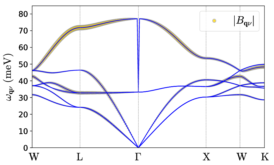
Phonon contributions to the exciton polarons in LiF. The size of the yellow discs represents the contribution from each individual phonon modes.
In the end, EPW will plot the electron and hole charge density isosurfaces for the exciton polaron through
ibrun -np 27 $QEPATH/epw.x -npool 27 -inp epw3.in > epw3.out
This step will take longer than the other two steps (around 10 minutes), but you can monitor the progress via
cat epw3.out
...
     Calculating the charge densities.
     Current progress:  0.01%
     Current progress: 10.06%
     Current progress: 20.13%
     Current progress: 30.15%
     Current progress: 40.14%
     Current progress: 50.37%
     Current progress: 60.29%
  ...
Two files, e_psir_plrn.xsf and h_psir_plrn.xsf will be generated, which contain the electron and hole charge density isosurfaces, respectively. You can first download them to your local computer via
scp username@frontera.tacc.utexas.edu:YOUR_WORK_DIR/"*_psir_plrn.xsf" .
and then open these two files using the software VESTA. You are expected to see electron and hole charge densities similar to fig_e_psir and fig_h_psir, respectively:
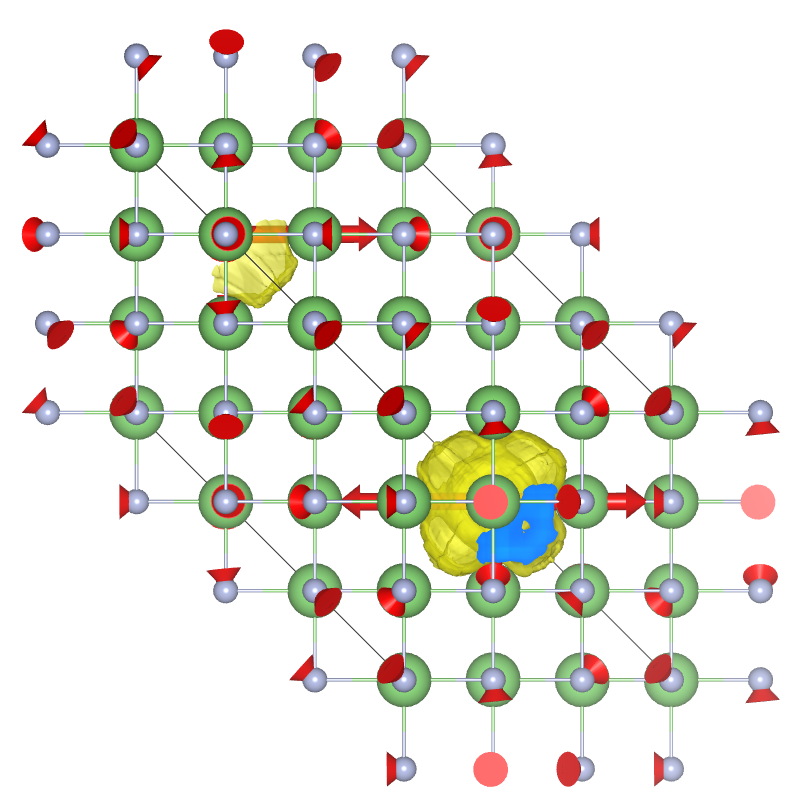
Electron charge density isosurface of the exciton polaron in LiF. The red arrows indicate the atomic displacements accompanying the charge densities.
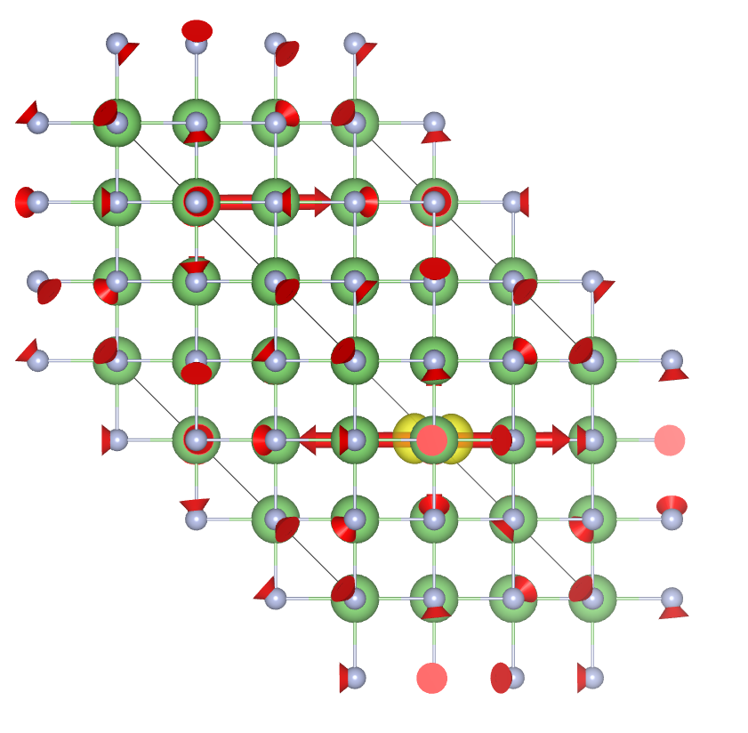
Hole charge density isosurface of the exciton polaron in LiF. The red arrows indicate the atomic displacements accompanying the charge densities.