B-doped Diamond
Warning
The following example aims at providing physically meaningful results. Calculations can therefore take a significant amount of time. For quick calculations, look at the EPW/tests/ folder.
Running EPW to calculate electron and phonon linewidths and the Eliashberg spectral function of B-doped diamond
The B-doped diamond example is located inside the EPW/examples/diamond/ directory. Within this directory there are three sub-directories: pp/ contains the C pseudopotential; phonon/ contains the input files to calculate phonons for B-doped diamond; epw/ contains the inputs to run epw.x on B-doped diamond.
Once pw.x, ph.x and epw.x have been compiled, we are ready to run this example.
The first step is to calculate phonons in the irreducible wedge. For this example we use a 6x6x6 coarse grid of phonon wavevectors. First go inside the phonon directory:
cd phonons
The phonon code from QE requires a ground-state self-consistent run
../../../../bin/pw.x < scf.in > scf.out
Note that all the calculations can also be performed in parallel using MPI, by issuing the following command:
mpirun -np N ../../../../bin/pw.x -npool N < scf.in > scf.out
where N must be replaced by the number of cores on which you wish run EPW. Since the current version of EPW does not support parallelization over planewaves G, N must be the same number in the specifications of -np and -npool. If you are using a HPC running a job scheduler, then you can embed the line above in your batch job script. If you are running pw.x, ph.x, and epw.x in parallel, please make sure to use the same number of cores in all calculations.
The electronic band structure of B-doped diamond is shown in Figure 1.
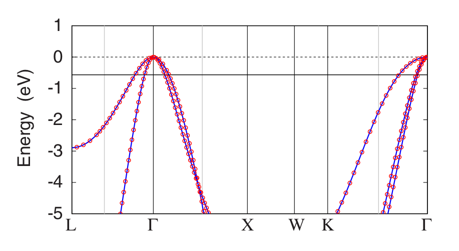
Figure 1: Comparison between the electronic band structure of pristine diamond (lines) and of B-doped diamond (circles). The Fermi level corresponding to a B concentration of 1.85% is located 0.57 eV below the top of the valence band, and is indicated by a solid black line. Image taken from Giustino et al, Phys. Rev. B 76, 165108 (2007).
Calculating phonons
We now continue with a sequential run. Let us compute the dynamical matrix, the phonon frequencies and the variations of the self-consistent potential using the ph.x code from QE. We issue the following command:
../../../../bin/ph.x < ph.in > ph.out
This provides us with the phonon frequencies and dynamical matrices at 16 irreducible q-points. You can now check that your results are consistent with the phonon dispersion relations shown in Figure 2.
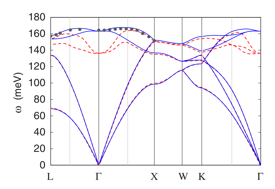
Figure 2: Comparison between the phonon dispersion relations of pristine diamond (solid lines) and B-doped diamond (dashed lines). The disks are inelastic neutron scattering data. Image taken from Giustino et al, Phys. Rev. B 76, 165108 (2007).
Now we need to copy the .dyn, .dvscf, and .phsave files which have been produced by QE inside the save folder. The files corresponding to the various q-points need to be relabelled by appending the q-point number in the list. This operation is performed by a small python script. You simply need to issue the following command from within the folder phonons/:
python pp.py
The script will ask you the prefix used for the QE calculations, as well as the number of irreducible q-points computed. The script will place all the files in the save/ folder. We can now move to the epw folder.
In preparation of the EPW run we need to compute the Kohn-Sham wavefunctions and eigenvalues on a coarse Brillouin zone grid. For this we perform first a scf calculation and then an nscf calculation. We move into the epw/ directory and issue:
../../../../bin/pw.x < scf.in > scf.out
mpirun -np N ../../../../bin/pw.x -npool N < nscf.in > nscf.out
Now we have all the information needed to run EPW.
Calculating electron and phonon linewidths using EPW
We start by computing the phonon linewidths,
that is the imaginary part of the phonon self-energy. This is achieved by using the setting phonselfen = .true. in the epw.in input file. The phonon linewidths are calculated for ‘’’q’’’-points included in the filed specified by the key filqf = 'meshes/path.dat' inside epw.in. In this example the wavevectors specified by the meshes/path.dat file are along the \(L \Gamma X\) lines of the diamond Brillouin zone.
If you want to generate alternative paths, you will find a python script called kgen.py inside the
folder meshes/. This script can be adapted to generate any path that you might need.
At this point we can run EPW:
mpirun -np N ../../../bin/epw.x -npool N < epw.in > epw.out
This run will create a number of files. Let us focus for now on the file linewidth.phself. This file contains the phonon linewidths (arising the electron-phonon interaction), along the high symmetry lines \(L \Gamma X\).
If you plot the last column, which corresponds to the highest-energy optical mode, you should obtain something very similar to Figure 3.
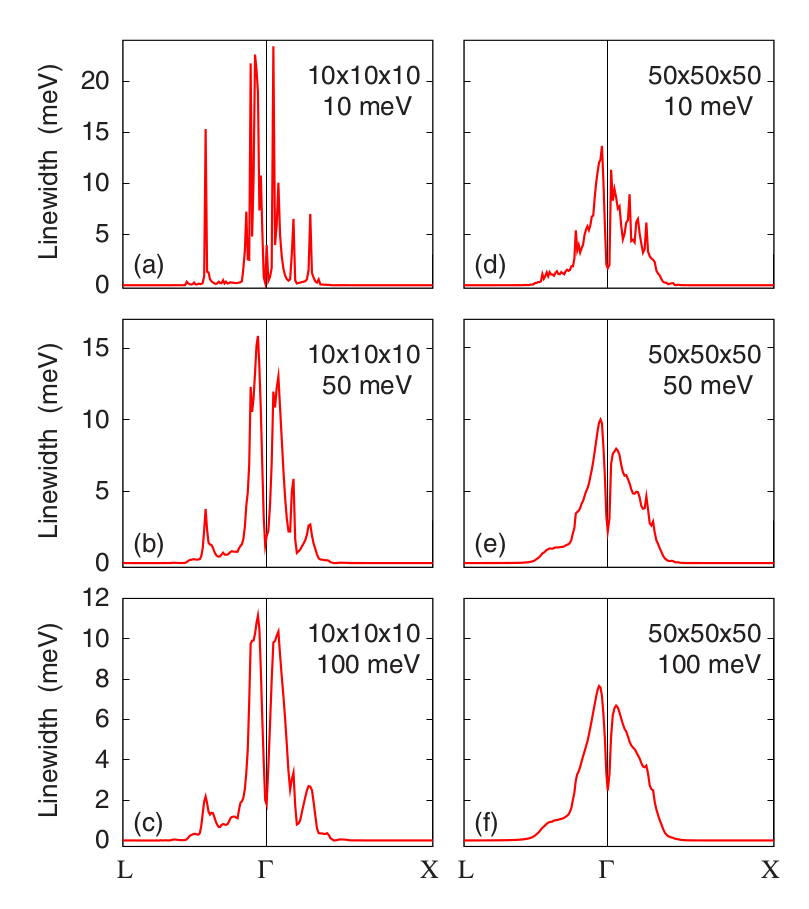
Figure 3: Calculated phonon linewidths for the highest optical mode of B-doped diamond. The density of k-points and the smearing parameter are reported in each panel. Image taken from Giustino et al, Phys. Rev. B 76, 165108 (2007).
The plots shown in Figure 3 were performed by using randomly-shifted grids. This choice makes all the k-points inequivalent. In the file epw.in we are specifying a homogeneous and unshifted k-grid with 50x50x50 points, which corresponds to 3107 inequivalent points. Using this choice we obtain the following plot:
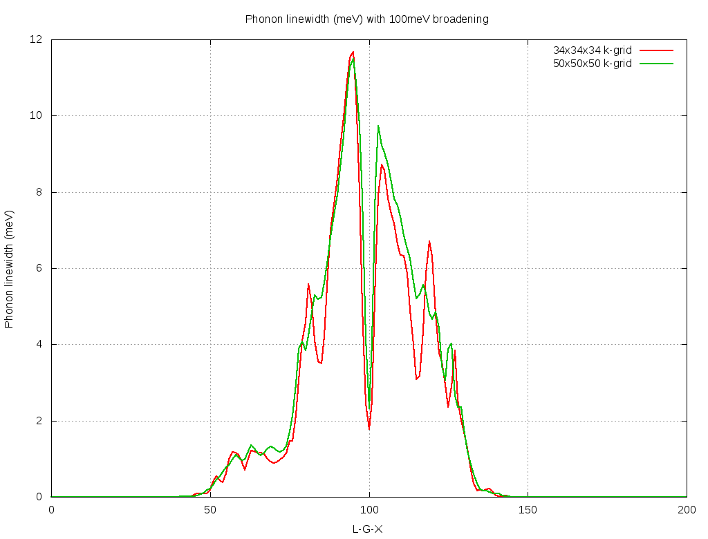
Figure 4: Calculated phonon linewidths for the highest optical mode of B-doped diamond. The k-point density and broadening parameters are indicated.
Reference output files can be found in the folder ref.out.
We now move to the ‘’’electron linewidths’’’.
In this case we must integrate over the phonon q-points. We therefore have to change the fine grid nqf1 and specify the file that contains the k-points for which we want to compute the linewidths, filkf. Additionally, since we are now considering only a subset of the k-points in the Brillouin zone, we cannot determine the Fermi level automatically, but we need to give this parameter in input. In this example we use the Fermi level obtained in the output file epw.out which we obtained above when computing the phonon linewidths. In pratctice we set the following input parameters in the file epw2.in:
efermi_read = .true.
fermi_energy = 13.209862
We then run EPW by issuing:
mpirun -np 4 ../../../bin/epw.x -npool 4 < epw2.in > epw2.out
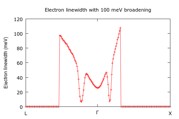
Figure 5: Calculated electron linewidths for the valence band of B-doped diamond, using a homogeneous and inshifted q-grid of 50x50x50 points.
Note that Fig. 9 of Giustino et al, Phys. Rev. B 76, 165108 (2007) corresponds to the electron linewidths evaluated for undoped diamond, hence they differ from the above result.
We can now compute the spectral function as the real and imaginary part of the electron self-energy arising from electron-phonon interactions:
In this expression we are taking \(\hbar=1\). In order to calculated the spectral function we issue the command:
../../../bin/epw.x < epw3.in > epw3.out
At the end of the run you should obtain the following spectral function, where the red lines are the Kohn-Sham eigenenergies.
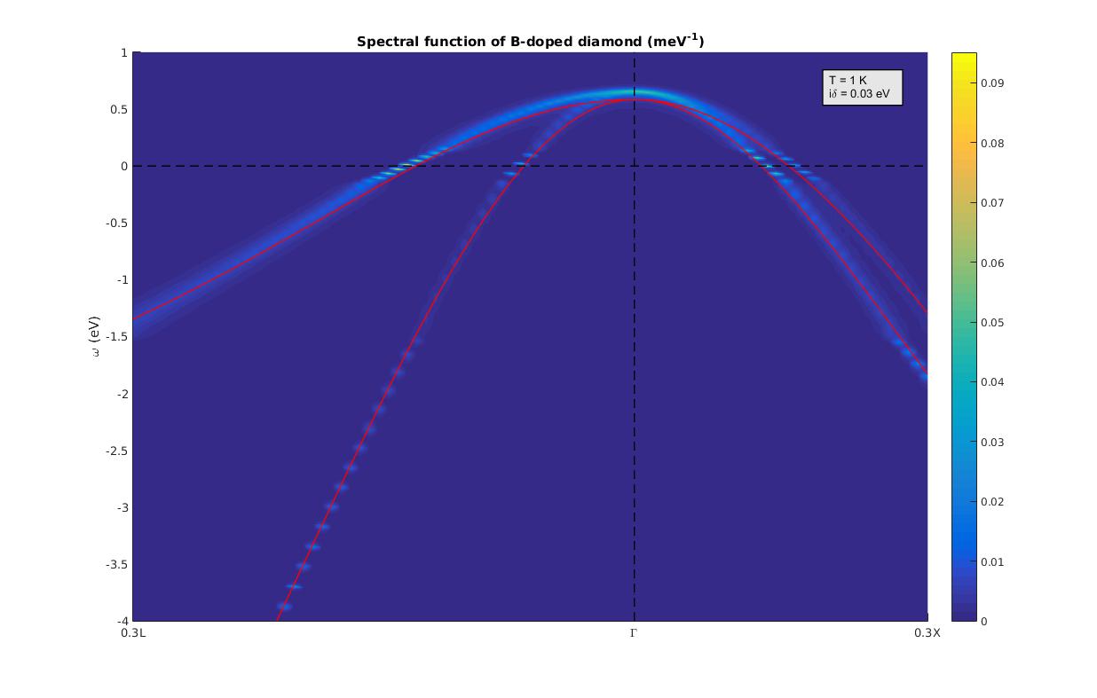
Figure 6: Calculated electronic spectral function for the valence band of B-doped diamond, on a 50x50x50 homogeneous and unshifted grid of q-points.
Technical note The real part of the self-energy requires also the calculation of the so-called Debye-Waller term, see for example Poncé et al, Phys. Rev. B 90, 214304 (2014). The current version of EPW only computes the Fan-Migdal self-energy. In the case of metals and doped semiconductors, the Debye-Waller term can be, in good approximation, be considered as a state-dependent constant, since it is real and frequency-independent..
In order to account for the Debye-Waller shift of the real part of the self-energy, as well as corrections beyond one-phonon processes, the EPW code enforces a sum rule to conserve the electron number (you can verify that the integral of the spectral function yields approximately 8, i.e. the number of electrons in this example):
The sum rule corresponds to requiring that the real part of the self-energy vanishes at the Fermi energy, and is enforced by default in EPW. The resulting spectral function is:
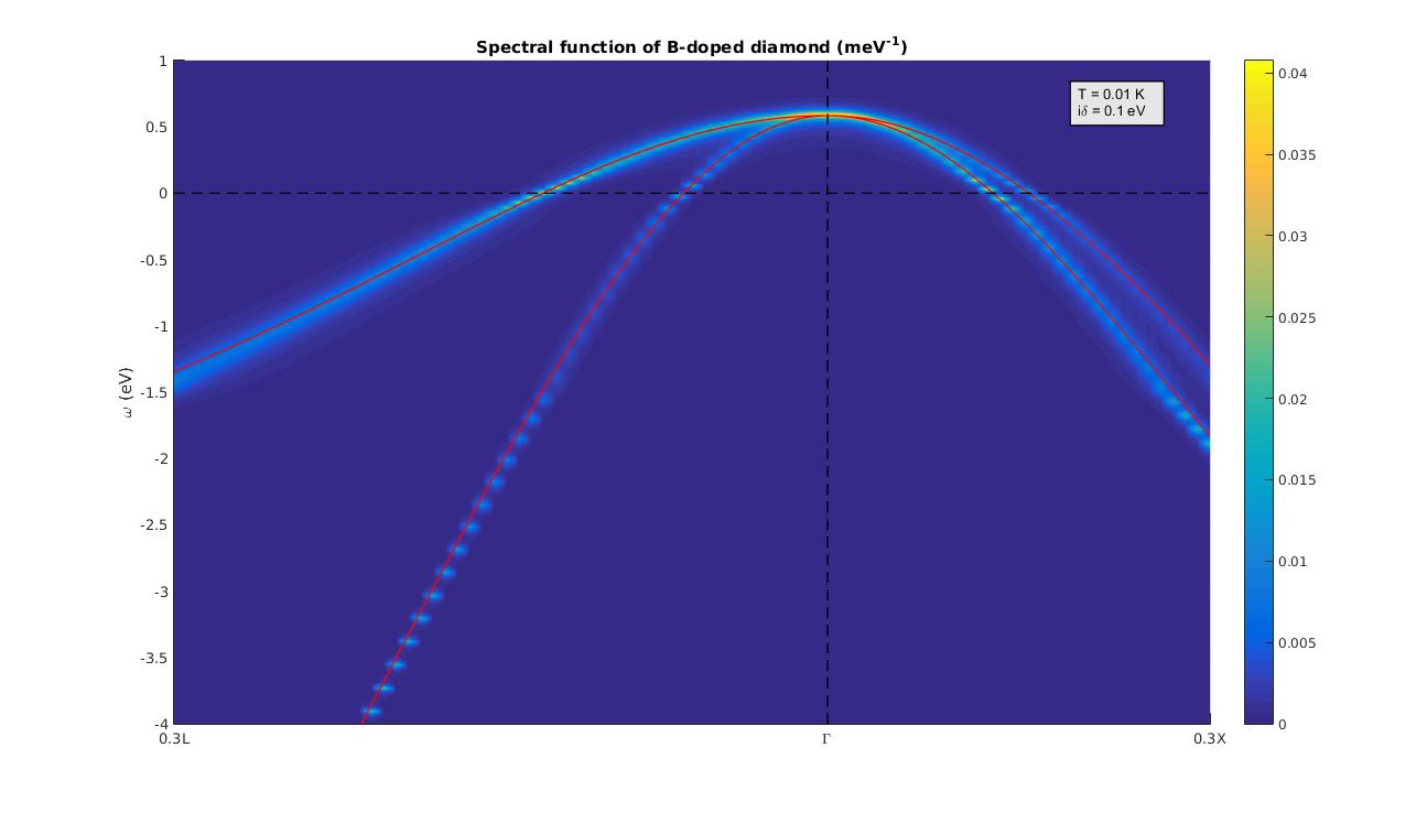
Figure 7: Calculated electronic spectral function for the valence band of B-doped diamond on a 50x50x50 homogeneous and unshidted grid of q-points.
We can also zoom closer to the Fermi level and see the narrowing of the linewidth, in agreement with Figure 5:
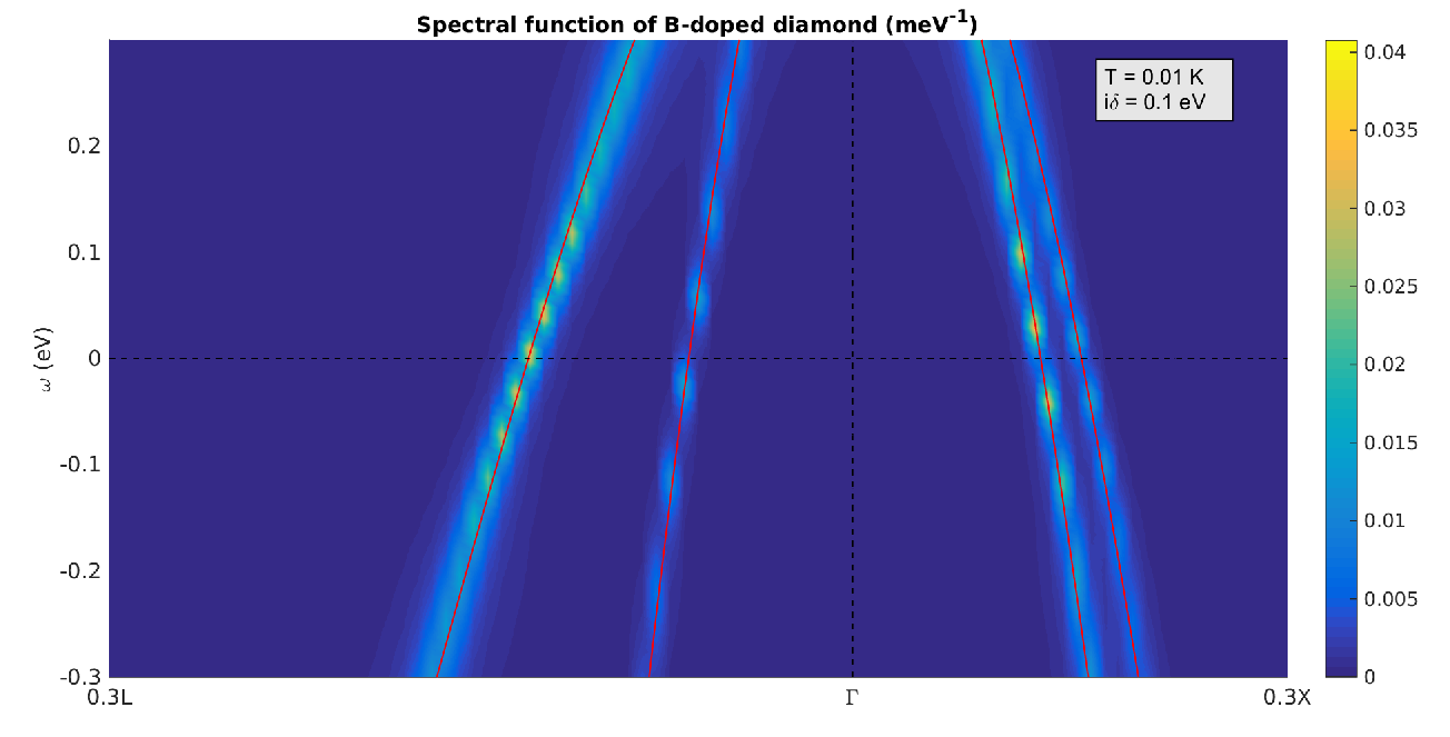
Figure 8: Electronic spectral function for the valence band of B-doped diamond: close-up of Figure 7 near the Fermi energy.
By increasing the k- and q-point resolution near the Fermi level it is also possible to observe the well-known band structure kinks.