FCC Lead
Author: Samuel Poncé
Warning
The following example aims at providing physically meaningful results. Calculations can therefore take a significant amount of time. For quick calculations, look at the EPW/tests/ folder.
Running EPW on bulk fcc Pb
The bulk fcc lead example is located inside the EPW/examples/pb/ directory. Within this directory there are three directories. pp/ contains the Pb pseudopotential, woSOC/ contains the input files to calculate the lead without spin-orbit coupling (SOC); wSOC contains the inputs files to run the lead calculations including SOC.
Once pw.x, ph.x and epw.x have been compiled, we are ready to run the example.
The first step is to calculate the phonons in the irreducible wedge. For this example, we use a 6x6x6 coarse grid.
First go inside the phonon directory of both woSOC/ and wSOC/ and issue
cd phonons
The phonon code from QE requires a ground-state self-consistent run
../../../../bin/pw.x < scf.in >& scf.out &
The electronic bandstructure of Pb is presented in Figure 1 below with and without SOC.
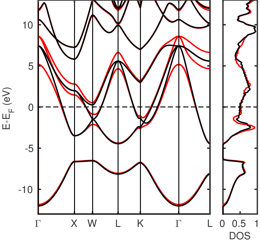
Figure 1: Electronic bandstructure and density of state (DOS) of Pb at the optimized lattice parameter with (red line) and without (black line) spin-orbit interaction. Image taken from [to be added].
Calculating the phonons
Let us compute the dynamical matrix, phonon frequencies and change of potential using the ph.x code
../../../../bin/ph.x < ph.in >& ph.out &
This will give us the phonon frequency and dynamical matrices at 16 irreducibles q-points. You can check that your results correspond to the phonon frequency of the Figure 2 below.
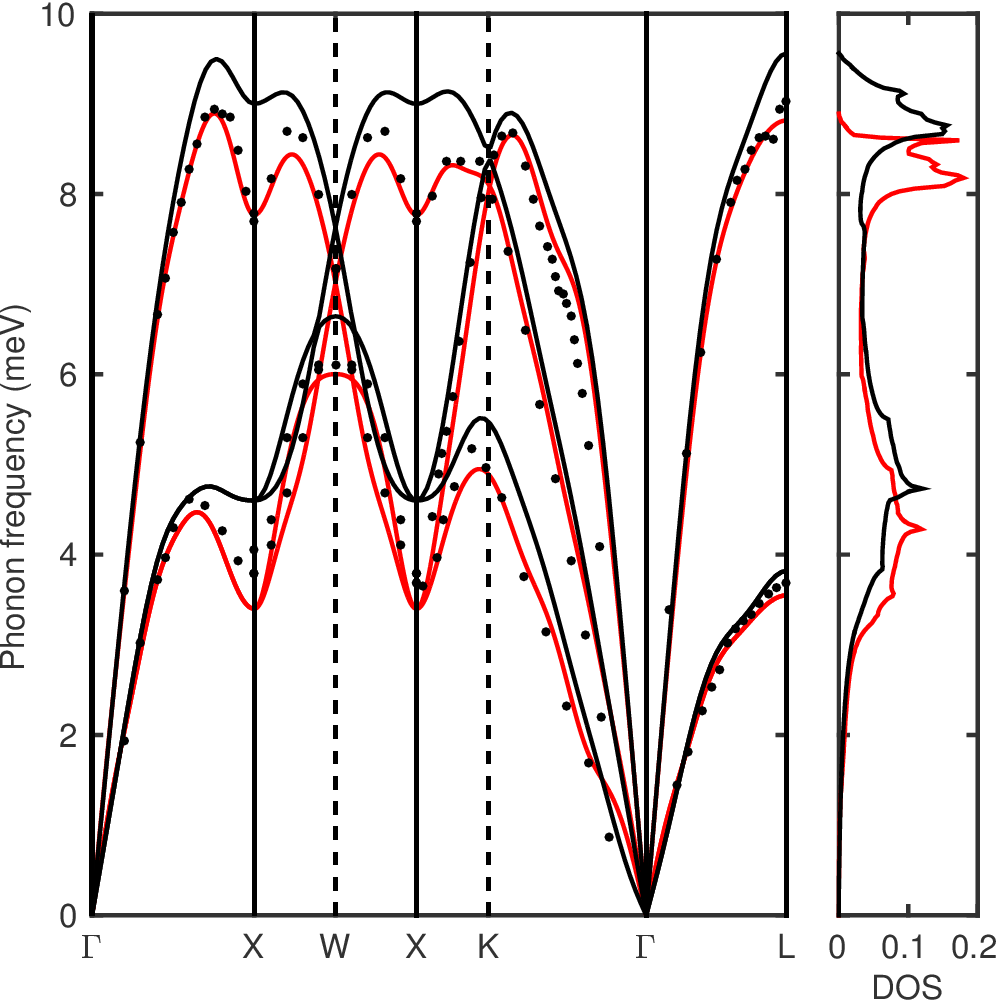
Figure 2: Phonon dispersion relation and density of state of Pb at the optimized lattice parameter with (red line) and without (black line) spin-orbit interaction. The calculations were done on a 14x14x14 k-point and a 10x10x10 q-point grid with a Gaussian broadening of 0.025~Ry. The experimental data (black dots) at 100 K from neutron spectrometry are taken from Brockhouse et al..
We then need to copy the .dyn and .dvscf as well as the _ph0/pb.phsave folder inside the save folder. Those are all the quantities produced by Quantum Espresso that EPW needs.
Because the files need to have a specific name and because there can be quite a few files, you can use the small python script to help you. Just issue
python pp.py
in the phonons folder. The script will ask you the prefix used for the QE calculations as well as the number of irreducible q-points computed. The script will place all the files in the save folder. We are now done with QE and can move to the epw folder.
Running EPW
We first have to do a scf and nscf calculations. To do that, go inside the epw directory and issue:
../../../../bin/pw.x < scf.in >& scf.out
../../../../bin/pw.x < nscf.in >& nscf.out
We can then run the EPW calculation. We will start by computing the phonon linewidth (imaginary part of the phonon self-energy). Note that we have set phonselfen = .true. in the epw.in input file.
We are here interested in the Eliashberg spectral function. For that you need to set a2f = .true..
You can then launch the EPW calculation:
../../../bin/epw.x < epw.in >& epw.out
The code should generate a file called pb.a2f.01. This file contains the Eliashberg spectral function \(\alpha^2F\) for different phonon smearing as a function of energy.
The convergence of this quantity with the k and q-point grid can be quite tedious in a material with a complex Fermi surface like Pb. See for example Figure 3 with and without SOC pseudopotential. These calculations are heavy and are not intended to be reproduced here. We gave it as an indication of the typical fine grid that might be required.
Also note that random k or q-point integration converges faster than homogeneous. To perform random integration, please refer to the input variables [[ Inputs#rand_q | rand_q ]] and [[ Inputs#rand_nq | rand_nq]].
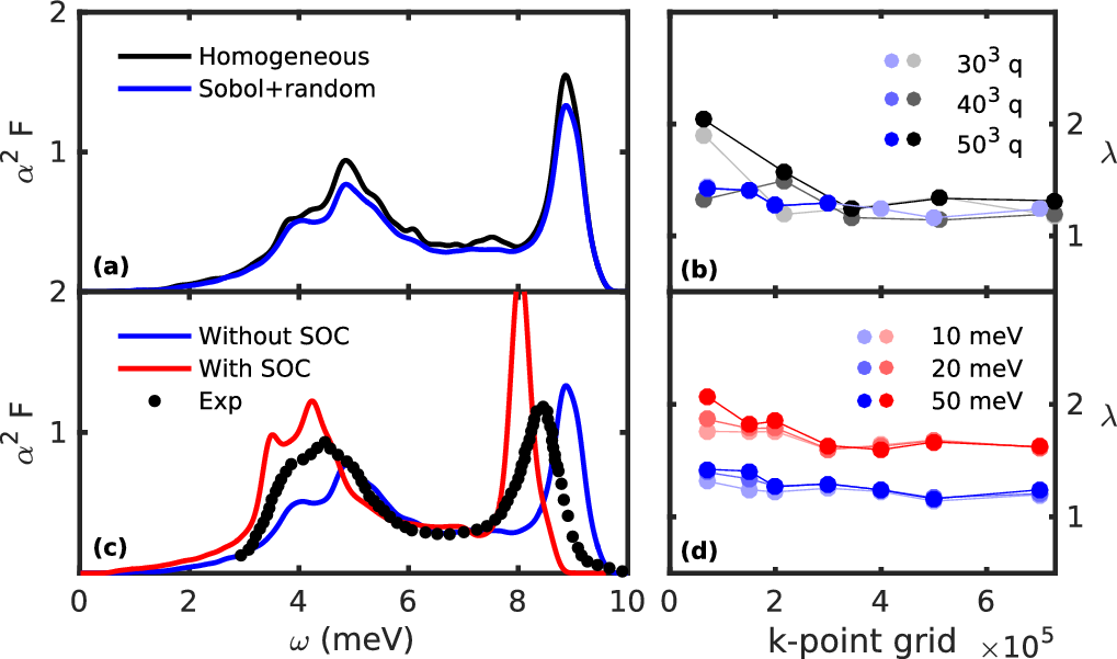
Figure 3: Effect of different fine sampling methods in EPW (homogeneous k and q-point integration against quasi random q-point using a Sobol algorithm) on (a) the Eliashberg \(\alpha^2F\) and (b) the electron-phonon coupling strength \(\lambda\) of Pb without SOC. Effect of the SOC on (c) the Eliashberg \(\alpha^2F\) with an electron smearing of 10 meV and (d) on \(\lambda\) when different electron smearing are considered. The phonon smearing is 0.15 meV. The experimental data points are taken from D. Scalapino, Superconductivity, Dekker, 1969.
Finally, the Figure 4 presents the calculated isotropic Eliashberg spectral function \(\alpha^2F(\omega)\) of Pb with and without SOC as well as its transport counterpart.

Figure 4: Calculated isotropic Eliashberg spectral function \(\alpha^2F(\omega)\) of Pb (blue solid line) and integrated electron-phonon coupling strength \(\lambda\) (thin blue solid line), compared with the Eliashberg transport function (blue dashed line) and the transport coupling strength \(\lambda_{tr}\) (thin dashed blue line). The same data are presented with spin-orbit coupling in red.
Note for expert users
If you wish to reproduce Figure 5 below (Pb resistivity using Ziman resistivity formula), you can use the python scripts from the following tar file
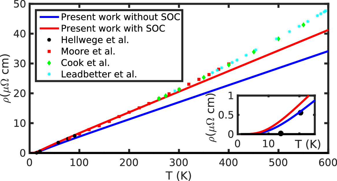
Figure 5: Calculated resistivity with (plain red line) and without (plain blue line) spin-orbit coupling. The inset shows a zoom of the resistivity on the 0-25~K temperature range.
The following video explain how to use the python script.
This video tutorial can also be found here.