GaN-II
Author: Samuel Poncé
Warning
The following tutorial is based on an automatic test from the test-suite and is intended to be run quickly. Careful convergence is required to obtain physically meaningful results.
Note
This is a new tutorial which include code features not yet available in the stable version of EPW/QE. Therefore you need the developer version to run it at the moment:
git clone https://gitlab.com/QEF/q-e.git
Linearised Boltzmann transport equation (BTE)
In this tutorial, we will show how to compute the intrinsic electron and hole mobility of hexagonal wurtzite GaN using the linearised iterative Boltzmann transport equation (IBTE) and the self-energy relaxation time approximation (SERTA).
The theory related to this tutorial can be found in the review First-principles calculations of charge carrier mobility and conductivity in bulk semiconductors and two-dimensional materials.
In particular the IBTE mobility refers to Eqs. 40, 41, 42 and 43 from the review while the SERTA mobility refers to Eqs. 41, 51 and 53. Note that an alternative formulation of the IBTE mobility is also given by Eqs. 63 and 64 by removing the magnetic field (B=0 limit).
In addition, the paper Towards predictive many-body calculations of phonon-limited carrier mobilities in semiconductors is the recommanded citation for the transport implementation in EPW.
Preliminary calculations
The tutorial files can be found in q-e/test-suite/epw_mob_polar which also include the pseudopotentials.
We first compute the dynamical matrix and electron-phonon matrix element using density functional perturbation theory on the irreducible Brillouin-Zone.
To do so, we first compute the ground-state electron density using 4 cores:
mpirun -np 4 ../../bin/pw.x < scf.in | tee scf.out
Note
For polar materials as is the case of GaN, the dielectric constant converges very slowly with the k-point grid (linearly). As a result, the k-point grid should be very dense (e.g. 20x20x20). In this example we use 2x2x2 for fast calculation.
We then compute the phonons:
mpirun -np 4 ../../bin/ph.x < ph.in | tee ph.out
Try looking in the ouput and locate the dielectric constants. You should get 23.12 in-plane and 17.23 for the out of plane direction. Those values are strongly overestimated due to the coarse k-point grid. The calculation should take about 5 min.
Note
The input variable responsible to produce the electron-phonon matrix element is fildvscf. Always make sure that this variable is present.
Finally, we need to post-process some of the data to make it ready for EPW. To do so, we can use the following python script
python ../../EPW/bin/pp.py
The script will ask you to enter the prefix used for the calculation. In this case enter “gan”. The script will create a new folder called “save” that contains the electron-phonon matrix elements and dynamical matrices on the IBZ.
The script should be compatible with python 2 and python 3.
Note
If you are using python 2, the script might ask you to install the “future” library. If so, type:
pip install --user future
For information, the converged phonon bandstructure of GaN should look like this:
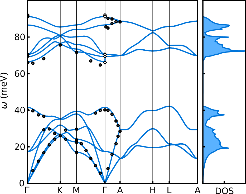
Figure 1: Phonon dispersion relations and phonon density of states of wurtzite GaN at the relaxed atomic positions. Figure from Poncé et al, Phys. Rev. B 100, 085204 (2019).
Interpolation of the electron-phonon matrix element in real-space with EPW
Because the earlier phonon calculation modified the density file, we have to do another DFT self-consistent calculation
mpirun -np 4 ../../bin/pw.x < scf.in | tee scf.out
Followed by a non-self consistent calculation
mpirun -np 4 ../../bin/pw.x -npool 4 < nscf.in | tee nscf.out
The reason for the non-self consistent calculation is that EPW needs the wavefunctions on the full BZ on a grid between 0 and 1.
Note
For the nscf calculation the number of pool -npool has to be the same as the total number of core -np
Note
Since we are also interested in electron mobility, we will need the conduction bands. Notice that we added the
input nbnd = 30 in nscf.in
We then run EPW:
mpirun -np 4 ../../EPW/src/epw.x -npool 4 < epw1.in | tee epw1.out
Note
The number of cores and pool have to be the same as for the nscf.in run.
The following EPW input variables are important in our case:
vme         = .true.      ! Compute exact velocities using Wannier interpolation
lpolar      = .true.      ! This is a polar material
lifc        = .false.     ! Do not use external IFC
asr_typ     = 'simple'    ! Use the simple acoustic sum rule
use_ws      = .true.      ! Use the optimal Wigner-Seitz cell
nbndsub     =  14         ! We Wannierize only 14 bands
nbndskip    =  12         ! We skip the first 12 bands
dvscf_dir   = './save/'   ! Directory where the save folder generated by the @pp.py@ python script is stored
band_plot   = .true.      ! We want to plot the electronic and/or phonon bandstructure (i.e. we do not use homogeneous fine grids)
filkf       = './MGA.txt' ! K-point path from M to Gamma to A
filqf       = './MGA.txt' ! Q-point path from M to Gamma to A
efermi_read = .true       ! Because our fine grids are non homogeneous, the code cannot determine the Fermi level
fermi_energy= 11.80       ! We need to provide the Fermi level manually.
fsthick     = 100.0       ! States that we want to take around the Fermi level. We want all states so we put a large value.@]
Note
Because our k and q coarse grid are so coarse, we need use_ws. However it makes the calculation heavier (more vectors).
If your fine grids are big enough (6x6x6 or more), you probably can use Gamma centered WS cell and use use_ws = .false.
Note
You can provide the k/q-point path either in crystal or Cartesian coordinate. To do that, modify the second element of the first line of the
MGA.txt file.
Note
To have an idea of which Fermi level you should use, you can first do a calculation with a homogeneous fine grids by removing filkf and filqf
and placing:
nk1   = 12
nk2   = 12
nk3   = 12
nq1   = 12
nq2   = 12
nq3   = 12
Finally, notice that at the end of epw1.in you need to provide the IBZ q-point list:
4 cartesian
0.000000000   0.000000000   0.000000000
0.000000000   0.000000000  -0.306767286
0.000000000  -0.577350269   0.000000000
0.000000000  -0.577350269  -0.306767286@]
This list has to be exactly the same as the one reported in the output of the phonon calculation at the begining of ph.out that we did earlier.
The calculation should take about 1 min to run. At the end, the code should have produce two files band.eig and phband.freq which contain
the interpolated electronic and phonon bandstructure along the M-G-A path.
You can post-process those file yourself or used the plotband tool from Quantum Espresso by typing
../../bin/plotband.x
Then follow the instruction. Read the plotband.x documentation if you have an issue. This will create a file which is
graphable with gnuplot and should give you the following:
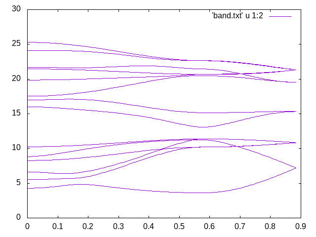
Figure 2: Wannierized electron bandstructure along the M-G-A path using EPW.
and the phonon bandstructure:
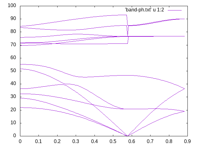
Figure 3: Wannierized phonon bandstructure along the M-G-A path using EPW.
Given that we have been using a 2x2x2 k-point and q-point grid and a low energy cut-off, such bandstructure quality is remarkable. Comparing with Figure 1, one can see that the only qualitative issue is related to the highest phonon-mode along the G-A direction, which improves with more converged results.
The electronic bandstructure can be compared to the following converged one:
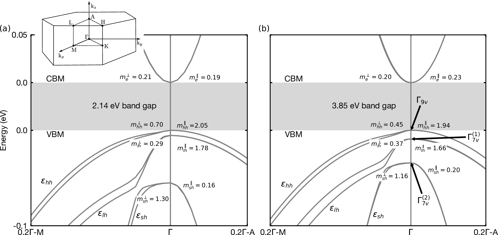
Figure 4: Electronic bandstructure of wurtzite GaN using (a) the LDA functional in the optimized ground-state LDA structure, and (b) quasiparticle G0W0 calculation. We indicate the effective masses at the zone center, obtained from the second derivatives of the band energy with respect to the wavevector along the ΓM and ΓA directions, respectively. The bandgap is off scale for clarity. We indicate the naming convention for the three topmost eigenstates at Γ. The energy levels have been aligned to the band edges. A schematic of the Brillouin zone of wurtzite GaN is given in the upper left corner. Figure from Poncé et al, Phys. Rev. B 100, 085204 (2019).
The main difference with the calculation that we just did is that we did not include SOC in this tutorial for speed reasons. You can add SOC by adding
noncolin        = .true.,
lspinorb        = .true.
in the scf.in and nscf.in files.
Calculating the intrinsic drift mobility tensor of GaN with temperature
We are now ready to compute the electron and hole mobility tensor with temperature. For this, run the following command to compute the hole mobility:
mpirun -np 8 ../../EPW/src/epw.x -npool 8 < epw2.in | tee epw2.out
In this case, the code does a restart by reading the electron-phonon matrix element in real-space from the file gan.epmatwp1 and interpolate the
matrix element on a fine k/q-point grid.
Note
In case of such a restart, you can use an arbitrary number of cores (.e.g. we used 8 instead of 4). The maximum you can use corresponds to the maximum number of k-points on the fine grid.
Before looking at the output, let us first discuss the specific input variable to perform transport calculations:
kmaps       = .true. ! Required for a restart
epwread     = .true. ! Tels the code to read the gan.epmatwp1 file
wannierize  = .false. ! The Wannierization cannot be redone for a restart

scattering    = .true.   ! We wish to compute scattering rates
iterative_bte = .true.   ! We wish to do IBTE and not just SERTA
mob_maxiter   = 200      ! Maximum number of iterations for the IBTE
broyden_beta  = 1.0      ! Linear mixing between iterations
int_mob       = .false.  ! We do not want to do electron and hole at the same time
carrier       = .true.   ! We want to specify carrier concentration
ncarrier      = -1E13    ! We want 1E13 carrier per cm^3. The negative sign means hole
mp_mesh_k     = .true.   ! Use k-point symmetry to reduce the calculation cost

restart      = .true.  ! We want to create restart point during the interpolation
restart_freq = 50      ! A restart point is created every 50 q-points
selecqread   = .false. ! If .true. allows for reading the q-points within the fsthick
epmatkqread  = .false. ! Once the transition probabilities have been written to file, allow for a restart to compute the mobilities

nstemp      = 2    ! We are considering 2 temperatures.
tempsmin    = 100  ! Initial temperature
tempsmax    = 300  ! Final temperature
degaussw    = 0.00 ! Broadening of the Dirac deltas in the BTE. A value of 0 means adaptative broadening.
Note
There is a starting global and unique Fermi level given by fermi_energy or computed by the code.
This Fermi level is used for initialization of quantities and energy window determination.
However the real Fermi level used for the transport calculation is determined automatically by the code depending on the
required carrier concentration and temperature. There can even be up to two such real Fermi level (for electron and hole).
We can take a look at the output of this second EPW calculation. We see the following:
Using uniform q-mesh:   12  12  12
Size of q point mesh for interpolation:       1728
Using uniform MP k-mesh:   12  12  12
Size of k point mesh for interpolation:        266
Max number of k points per pool:               34
which tells us that we have a q-point grid with 1728 q-points (no symmetry) and a k-point grid with 266 k-points (IBZ). Since we are doing a parallelization on k-point, we will have 34 k-points per core.
Next, the code will try to reduce the number of q-points we need to compute by taking the one that contribute to the
energy window. A file called selecq.fmt will be created and can be read later to avoid recomputing.
Number selected, total             50            148
Number selected, total            100           1443
Number selected, total            150           1715
We only need to compute      162 q-points
The code then reports the VBM and CBM as well as the Fermi level for the hole calculation for each temperature:
Valence band maximum    =  11.381872 eV
Conduction band minimum =  13.076046 eV

Temperature  100.000 K
Mobility VB Fermi level =  11.517589 eV

Temperature  300.000 K
Mobility VB Fermi level =  11.804356 eV
The code also reports which states are included given the energy window:
Fermi Surface thickness =   0.400000 eV
This is computed with respect to the fine Fermi level  11.481872 eV
Only states between  11.081872 eV and  11.881872 eV will be included
The code then computes the transition probabilities but only saves the one that are large enough:
Save matrix elements larger than threshold: 0.372108862978E-23
Note that the threshold is computed automatically based on the size of the system and is very conservative. The total error made by neglecting those matrix elements is lower than machine precision.
Because we are using adaptive smearing, the code reports the min and maximum value of broadening for that q-point.
This information is printed every restart_freq.
Progression iq (fine) =         50/       162
Adaptative smearing = Min:     1.414214 meV
                      Max:   293.598353 meV
Progression iq (fine) =        100/       162
Adaptative smearing = Min:    28.908200 meV
                      Max:   319.312222 meV
Progression iq (fine) =        150/       162
Adaptative smearing = Min:    48.994246 meV
                      Max:   149.060946 meV
At the end all the transition probabilities are stored in the file gan.epmatkq1 as well as the support files sparsei,
sparsej, sparsek, sparseq and sparset. Note that the file size is 28 Kb, orders of magnitude smaller than
without matrix element threshold.
Note
The interpolation and storing of transition probabilities to file can take a lot of time. If the calculation crashes
during runtime (due to time-out for example), just put selecqread == .true. `` to avoid recomputing the ``selecq.fmt
and relaunch. The code will automatically continue.
Once all the transition probabilities are compute, you can always restart the calculation by using the epmatkqread == .true.
Note that here the code did that for you automatically:
epmatkqread automatically changed to .TRUE. as all scattering have been computed.
Then the code computes the SERTA mobility:
=============================================================================================
  Temp     Fermi   Hole density  Population SR                  Hole mobility
   [K]      [eV]     [cm^-3]      [h per cell]                    [cm^2/Vs]
=============================================================================================

100.000  11.5176   0.10000E+14   0.12925E-25    0.767956E-02    0.000000E+00    0.000000E+00
                                                0.000000E+00    0.767956E-02    0.000000E+00
                                                0.000000E+00    0.000000E+00    0.573540E+04
300.000  11.8044   0.10000E+14   0.00000E+00    0.585711E+01    0.000000E+00    0.000000E+00
                                                0.000000E+00    0.585711E+01    0.000000E+00
                                                0.000000E+00    0.000000E+00    0.184230E+03
The GaN in-plane mobility (xx and yy components) is 0.767956E-02 and the out-of plane one (zz) is 0.573540E+04. Those values are totally not converged and physically wrong because of the very coarse fine grids that we used. Typical grids are larger than 100x100x100. One would always expect the mobility at higher temperature to be lower than at low temperature. This is correctly the case of the out-of plane component but not for the in-plane.
Note
The population sum-rule is simply the sum of all change of population due to external electric field which should be 0. If this value is large, there is probably something wrong in the calculation.
Finally, the code starts solving the IBTE and converges after 36 iterations to:
Iteration number:        36


=============================================================================================
  Temp     Fermi   Hole density  Population SR                  Hole mobility
   [K]      [eV]     [cm^-3]      [h per cell]                    [cm^2/Vs]
=============================================================================================

 100.000  11.5176   0.10000E+14  -0.12824E-25    0.896091E-02    0.000000E+00    0.000000E+00
                                                 0.000000E+00    0.896091E-02    0.000000E+00
                                                 0.000000E+00    0.000000E+00    0.374318E+04
 300.000  11.8044   0.10000E+14   0.13235E-22    0.757728E+01    0.000000E+00    0.000000E+00
                                                 0.000000E+00    0.757728E+01    0.000000E+00
                                                 0.000000E+00    0.000000E+00    0.185868E+03

                                                 0.806237E-06    Max error
To conclude this tutorial, we launch the last calculation with:
mpirun -np 8 ../../EPW/src/epw.x -npool 8 < epw3.in | tee epw3.out
In this case, we compute the electron mobility.
Take some time to analyse the differences between epw3.in and epw2.in to understand how to do such calculations.
It should be quite self-explanatory.
For information, by using much denser grids as well as SOC and GW corrections on the eigenvalues, one can get a fair agreement with experiment as shown on the following figure:
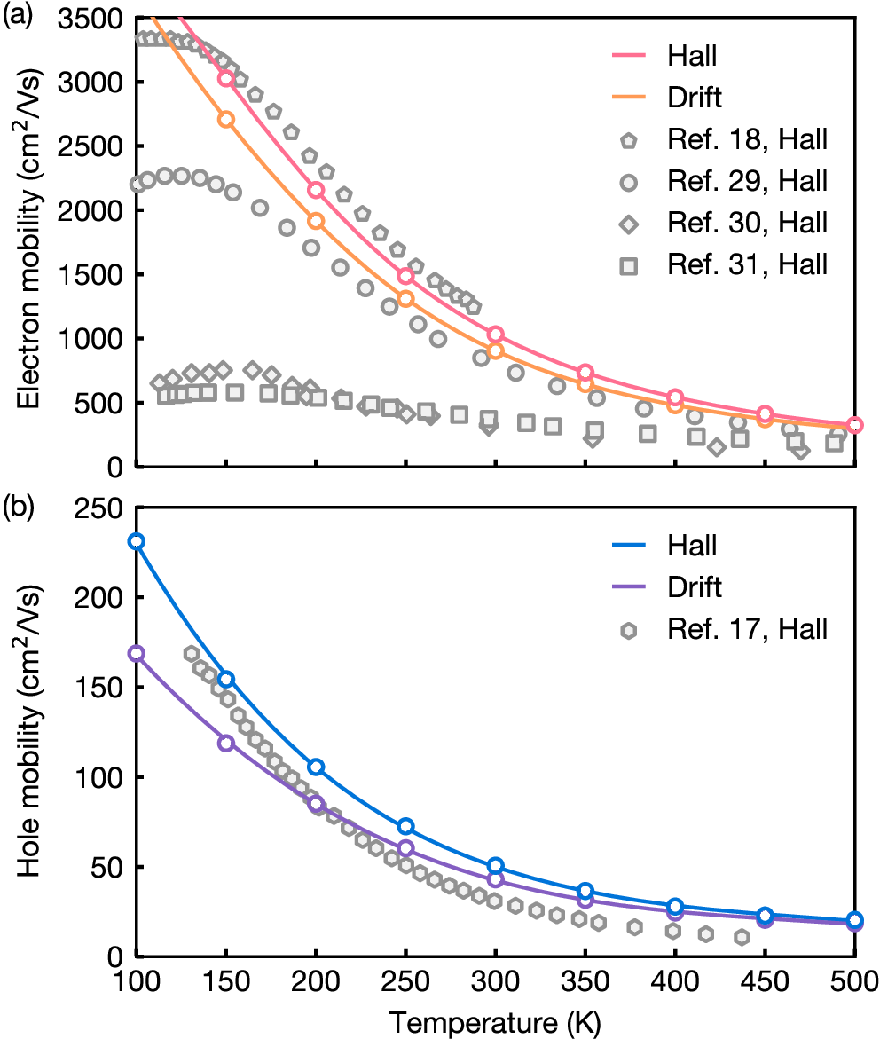
Figure 5: Electron (a) and hole (b) mobilities of wurtzite GaN, calculated using the IBTE, compared with the experimental data. We show both the drift mobilities and the Hall mobilities obtained by applying the Hall factor (not discussed here). Figure from Phys. Rev. Lett. **123**, 096602 (2019).
Suggestions for efficient transport calculations
Transport calculation are computationally heavy as they require a very fine sampling of both the k-point and q-point grids. However, various schemes have been implemented in EPW to reduce the computational cost.
1) The memory scales linearly with the number of temperature nstemp. Try decreasing it if you have memory issues.
The cpu times scales strongly sub-linearly with the number of temperature. Therefore try to do as many temperatures as your memory allows.
2) Low temperatures span a smaller energy window and are therefore more difficult to converge. You can decrease fsthick to make the
calculation more efficient. Note however that a single fsthick is used for all temperature so that your fsthick needs to be large
enough to accommodate the largest temperature.
3) Using int_mob == .true. is convenient because it allows for the calculation of both electron and hole at the same time.
However, the code consider only the element within an energy window given by fsthick around the starting Fermi level given by fermi_energy. As a result you might need to use a larger than needed fsthick. The recommended way is therefore to compute
electron and hole mobility in two separate runs.
4) Transport properties only require states very close to the band edge and significant speedup can be achieved
by using a small fsthick. Note that you need to converge your result with increasing values of fsthick and that larger values
are required for higher temperature. For example in this tutorial we used a 0.4 eV fsthick but we placed our Fermi level
0.1 eV above the valence band maximum (VBM). As a result we are considering only the states up to 0.3 eV above the VBM.
This is a typical order of magnitude.