GaN
Author: Samuel Poncé
Warning
The following example aims at providing physically meaningful results. Calculations can therefore take a significant amount of time. For quick calculations, look at the EPW/tests/ folder.
Running EPW on polar wurtzite GaN
The polar wurtzite GaN example is located inside the EPW/examples/gan/ directory. Within this directory there are three directories. pp/ contains the Pb pseudopotential, phonon/ contains the input files to calculate the phonons for GaN; epw/ contains the inputs to run epw.x on GaN.
Once pw.x, ph.x and epw.x have been compiled, we are ready to run the example.
Calculating the phonons
The first step is to calculate the phonons in the irreducible wedge. For this example, we use a 6x6x6 coarse grid.
First go inside the phonon directory
cd phonons
The phonon code from QE requires a ground-state self-consistent run
../../../../bin/pw.x < scf.in >& scf.out &
The electronic bandstructure of w-GaN is presented in Figure 1 below.
We will now continue in sequential. Let us compute the dynamical matrix, phonon frequencies and change of potential using the ph.x code
../../../../bin/ph.x < ph.in >& ph.out &
This will give us the phonon frequency and dynamical matrices at 28 irreducibles q-points.
We then need to copy the .dyn and .dvscf as well as the _ph0/diam.phsave folder inside the save folder. Those are all the quantities produced by Quantum Espresso that EPW needs.
Because the files need to have a specific name and because there can be quite a few files, you can use the small python script to help you. Just issue
python pp.py
in the phonons folder. The script will ask you the prefix used for the QE calculations as well as the number of irreducible q-points computed. The script will place all the files in the save folder. We are now done with QE and can move to the epw folder.
The phonon bandstructure of w-GaN is presented in Figure 1 below.
Calculating the electron-phonon matrix element using EPW
We first have to do a scf and nscf calculations. To do that, go inside the epw directory and issue:
../../../../bin/pw.x < scf.in >& scf.out
../../../../bin/pw.x < nscf.in >& nscf.out
We can then run the EPW calculation. We will start by computing the phonon linewidth (imaginary part of the phonon self-energy). Note that we have set phonselfen = .true. in the epw.in input file.
Also you can notice that we are computing the interpolated electron-phonon matrix element along the high-symmetry q-point line. This is achieved by reading a data file using the filqf = 'gan_band.qpt' input command.
You can then launch the EPW calculation:
../../../bin/epw.x < epw.in >& epw.out
Although the electron-phonon matrix elements as presented at the bottom of Figure 1 are not outputted directly (usually not relevant), you can easily print them by modifying the code. This should give you the correct red interpolation line as seen on the figure.
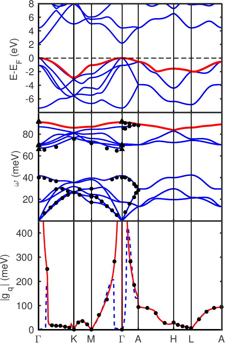
Figure 1: (Top) Electronic bandstructure of w-GaN along high-symmetry line of the Brillouin zone. The red line is the considered band in the bottom figure. (Middle) Phonon dispersion interpolated from a 6x6x6 \(\Gamma\)-centered q-point grid. The red line is the considered optical mode in the bottom figure. The filled disk are single crystal inelastic X-ray scattering data~ T. Ruf et al. and the filled diamond are Raman data~ H. Siegle et al.. (Bottom) Calculated electron-phonon matrix elements at \(\mathbf{k}-\Gamma\) for the highest band and mode index starting from a 6x6x6 electron and phonon grids. The gauge-invariant \(|g_{\mathbf{q}}|\) is averaged over degenerated states. The blue dashed line shows the standard interpolation and the red line shows the correct polar interpolation. The two are compared with direct DFPT calculations at each wavevector (filled discs).