Superconducting magnesium diboride

Warning

The following example aims at providing physically meaningful results. Calculations can therefore take a significant amount of time. For quick calculations, look at the EPW/tests/ folder.

Running EPW to calculate the anisotropic superconducting gap of MgB₂

This example is based on the papers Phys. Rev. B 87, 024505 (2013) and arXiv:1604.03525, which you should check for the physical interpretation of the results and a description of the main equations used in this tutorial.

The MgB₂ example is located inside the EPW/examples/mgb2/ directory. Within this directory you will find three subdirectories: pp/ contains the Mg and B pseudopotentials; phonon/ contains the input files needed for calculating the phonon dispersions of MgB₂; epw/ contains the input files to run epw.x on MgB₂ .

Once epw.x has been compiled, we are ready to run the example.

Calculating phonons

The phonon code of QE requires a ground-state self-consistent calculation:

../../../../bin/pw.x < scf.in >& scf.out &

The electronic bandstructure of MgB₂ is shown in Figure 1 below.

We will now proceed with a sequential run. Let us compute the phonon frequencies and eigenmodes using ph.x:

../../../../bin/ph.x < ph.in >& ph.out &

This will provide us with the files containing the dynamical matrices and the variations of the self-consistent potentials at 28 irreducibles q-points. We now need to copy the .dyn and .dvscf files, as well as the _ph0/diam.phsave folder, inside the save/ folder. These files contain all the information that EPW needs from Quantum Espresso.

EPW expect these files to be labelled according to the number of the irreducible q-point in the list. In order to label the files correctly you can use the python script pp.py. If you decide to proceed this way, just issue the statement:

python pp.py

from within the phonon/ folder. The script will ask you the prefix used for the QE calculations as well as the number of irreducible q-points computed. The script will rename all the required files and place them in the folded save/. At this point we are done with QE and can move to the epw folder.

The phonon dispersion relations of MgB₂ are shown in Figure 1 below.

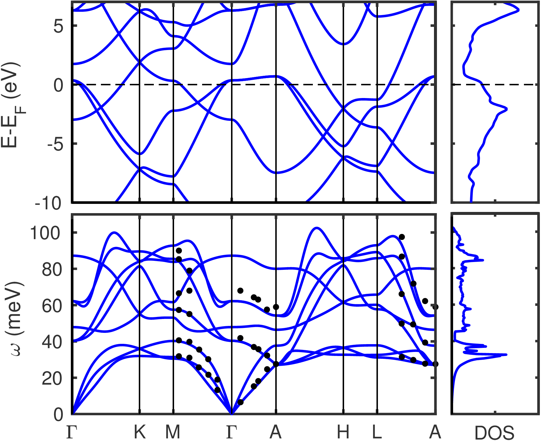
Figure 1: Electronic band structure and DOS of bulk MgB₂ (top), as well as phonon dispersion relations and PDOS (bottom). The calculations are executed using the experimental lattice parameters. The inelastic X-ray scattering data (black dots) at 300~K are from A. Shukla et al..

Running EPW

We first have to perform one scf and one nscf calculation. To do this, we go inside the epw directory and issue:

../../../../bin/pw.x < scf.in >& scf.out

../../../../bin/pw.x < nscf.in >& nscf.out

You can then launch the EPW calculation:

../../../bin/epw.x < epw.in >& epw.out

The calculation of superconducting properties is triggered by the flag eliashberg  = .true. and will be accompanied by significant I/O. In the following we describe the various output files, and we will use XX to indicate the temperature at which the anisotropic gap equations are solved. Please note that the figures shown below have been generated using denser Brillouion zone grids than those indicated in the example input files.

• MgB2.a2f

  This file contains the Eliashberg spectral function as a function of frequency \(\omega\) (meV), calculated using various smearing parameters (see Figure 2 below).

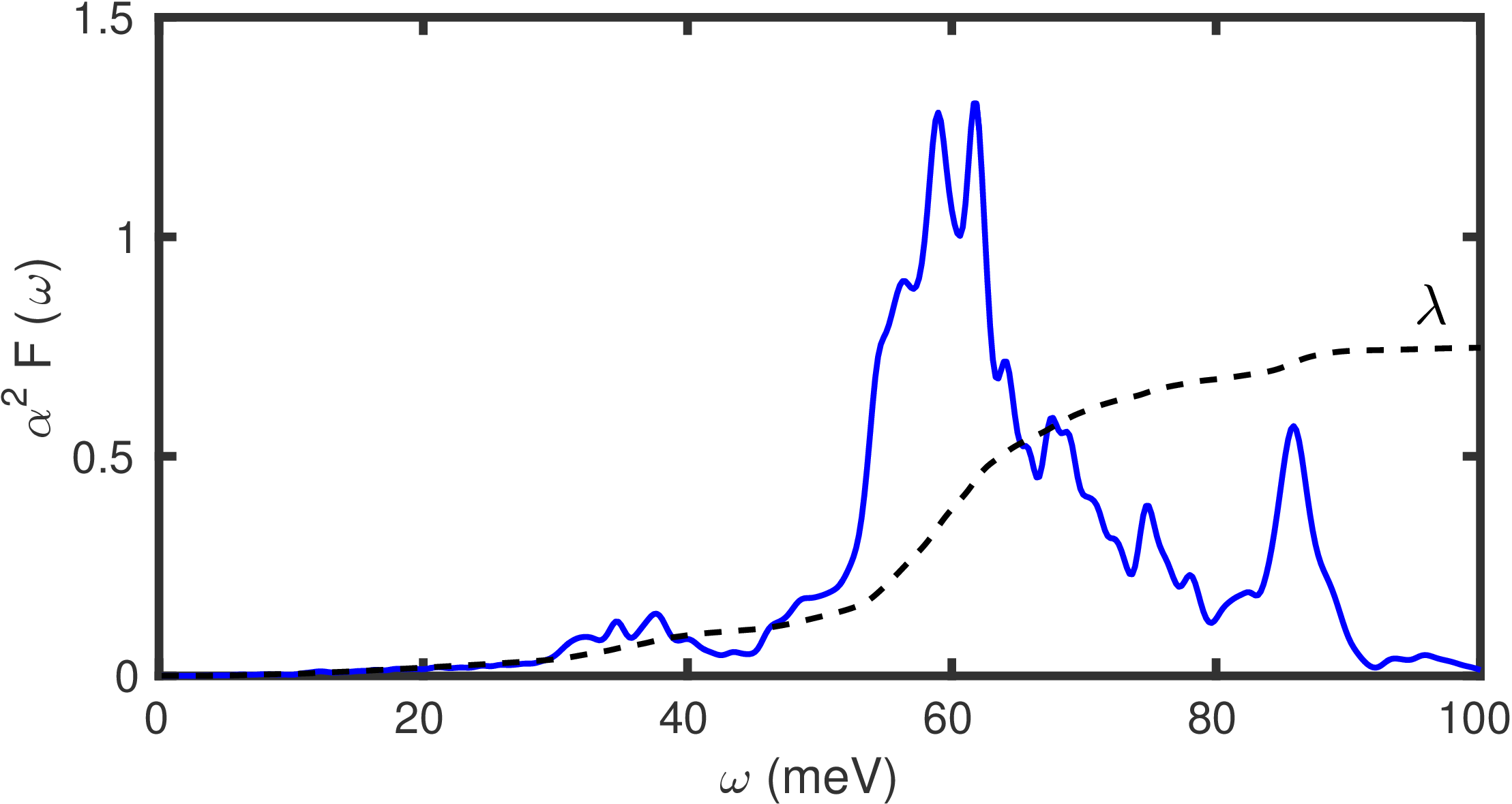
Figure 2: Calculated isotropic Eliashberg spectral function \(\alpha^2 F(\omega)\) of MgB₂ (blue solid line), and cumulative electron-phonon coupling strength \(\lambda\) (black dashed line). The results are integrated on a homogeneous fine k-point grid containing 60x60x60 points, and a fine homogeneous q-mesh with 30x30x30 points.

• MgB2.a2f_iso

  This file contains the Eliashberg spectral function as a function of frequency \(\omega\) (meV) . The second column is the Eliashberg spectral function corresponding to the first smearing value in MgB2.a2f. The remaining columns in MgB2.a2f_iso (3 x number of atoms) contain the mode-resolved Eliashberg spectral function (there is no specific information on which modes correspond to which atomic species).

• MgB2.phdos

  This file contains the total phonon density of states as a function of frequency \(\omega\) (meV) calculated using various smearing parameters. The smearing values are the same as in MgB2.a2f.

• MgB2.phdos_proj

  This file contains the phonon density of states as a function of frequency \(\omega\) (meV). The second column is the total phonon density of states corresponding to the first smearing value in MgB2.phdos. The remaining columns in MgB2.phdos_proj (3 x number of atoms) contain the mode-resolved phonon density of states (there is no specific information on which modes correspond to which atomic species).

• MgB2.imag_aniso_XX

  This file contains 5 columns: the frequency along the imaginary-axis \(\omega\) (eV), the Kohn-Sham eigenvalue \(E_{n{\bf k}}\) for band \(n\) and wavevector \({\bf k}\) relative to the Fermi energy (eV), the quasiparticle renormalization \(Z_{n{\bf k}}\), the superconducting gap \(\Delta_{n{\bf k}}\) (eV), and the quasiparticle renormalization \(Z_{n{\bf k}}\) in the normal state. The gap is shown in the top panel of Figure 3 below.

• MgB2.pade_aniso_XX

  This file contains similar information as in MgB2.imag_aniso_XX, but the superconducting gap is along the real axis and is obtained via Pade approximants. This file is written if iverbosity=2 in the input file, and the result is shown in the lower panel of Figure 3 below.

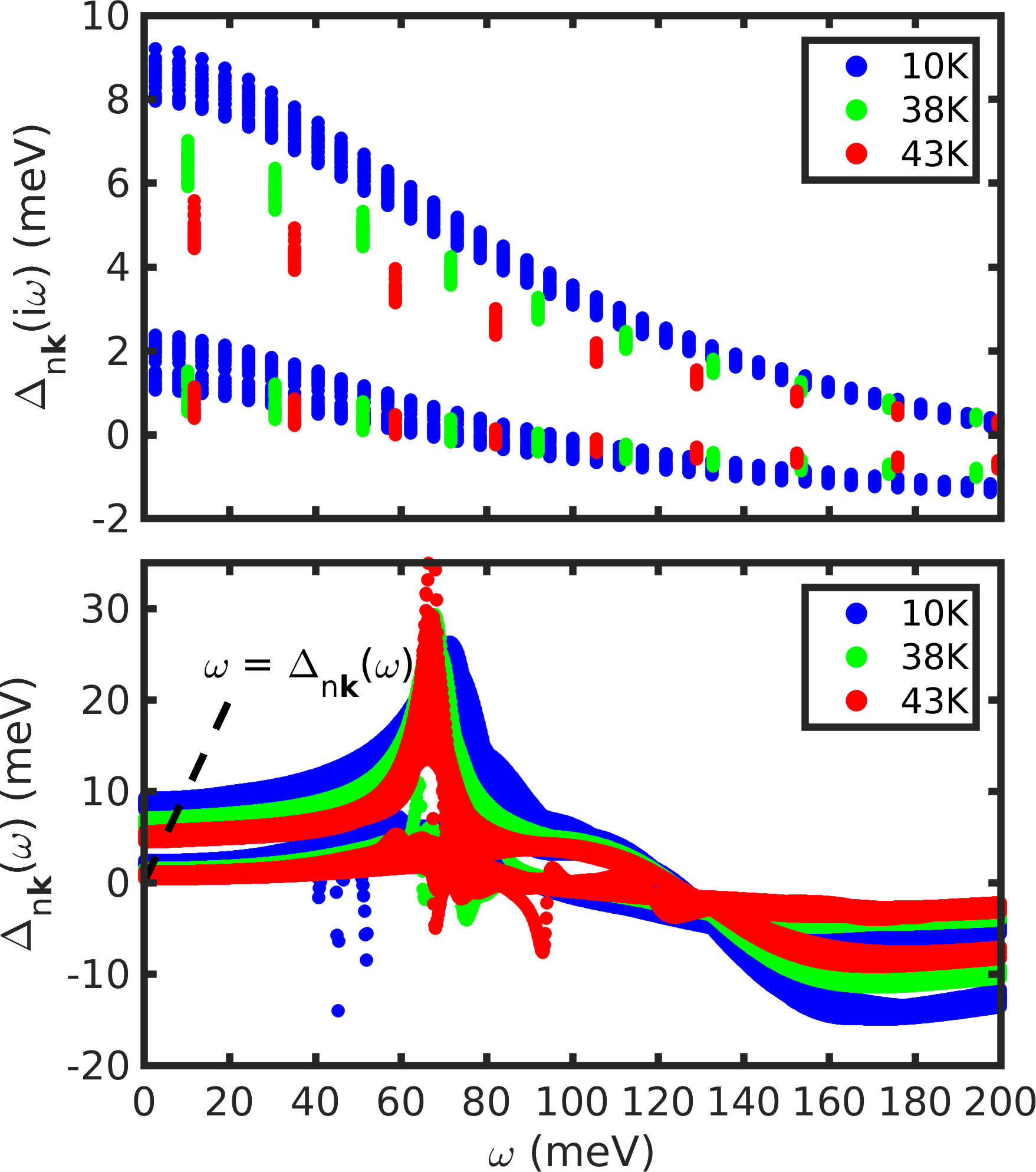
Figure 3: Calculated energy-dependent superconducting gap of MgB₂ from the anisotropic Eliashberg theory, at 10~K (blue), 38~K (green) and 43~K (red). The upper panel shows the gap along the imaginary energy axis, the lower panel is along the real energy axis (approximate analytic continuation via Padé functions. Only the KS states n**k** with an energy within 0.1~eV from the Fermi level are shown.

• MgB2.imag_aniso_gap0_XX

  This file contains the distribution of the anisotropic superconducting gap \(\Delta_{n{\bf k}}(\omega=0)\) (eV) on the Fermi surface, as obtained from the imaginary-axis calculation.

• MgB2.pade_aniso_gap0_XX

  This file contains similar information as in MgB2.imag_aniso_gap0_XX, but in this case the gap is calculated on the real axis using Padé approximants. This is shown in Figure 4 below.

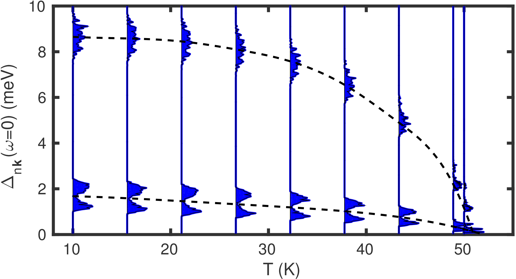
Figure 4: Calculated anisotropic superconducting gap \(\Delta_{n\mathbf{k}}(\omega=0)\) of MgB₂ on the Fermi surface, evaluated as a function of temperature. The superconducting gaps are obtained from the aproximate analytic continuation using Padé functions, and the Coulomb potential is set to \(\mu_c^*=0.16\). For each temperature the histograms indicate the number of states on the Fermi surface with that superconducting gap energy. The dashed lines are guides to the eye. The two superconducting gaps vanish at the calculated critical superconducting temperature \(T_{\rm c}\) of 51~K [note this value is about 30% higher than in the experiment].

• MgB2.qdos_XX

  This file contains the quasiparticle density of states in the superconducting state, relative to the DOS in the normal state, \(N_{\rm S}(\omega)/N_{\rm N}(\omega)\) as a function of frequency \(\omega\) (eV). This is shown in Figure 5 below.

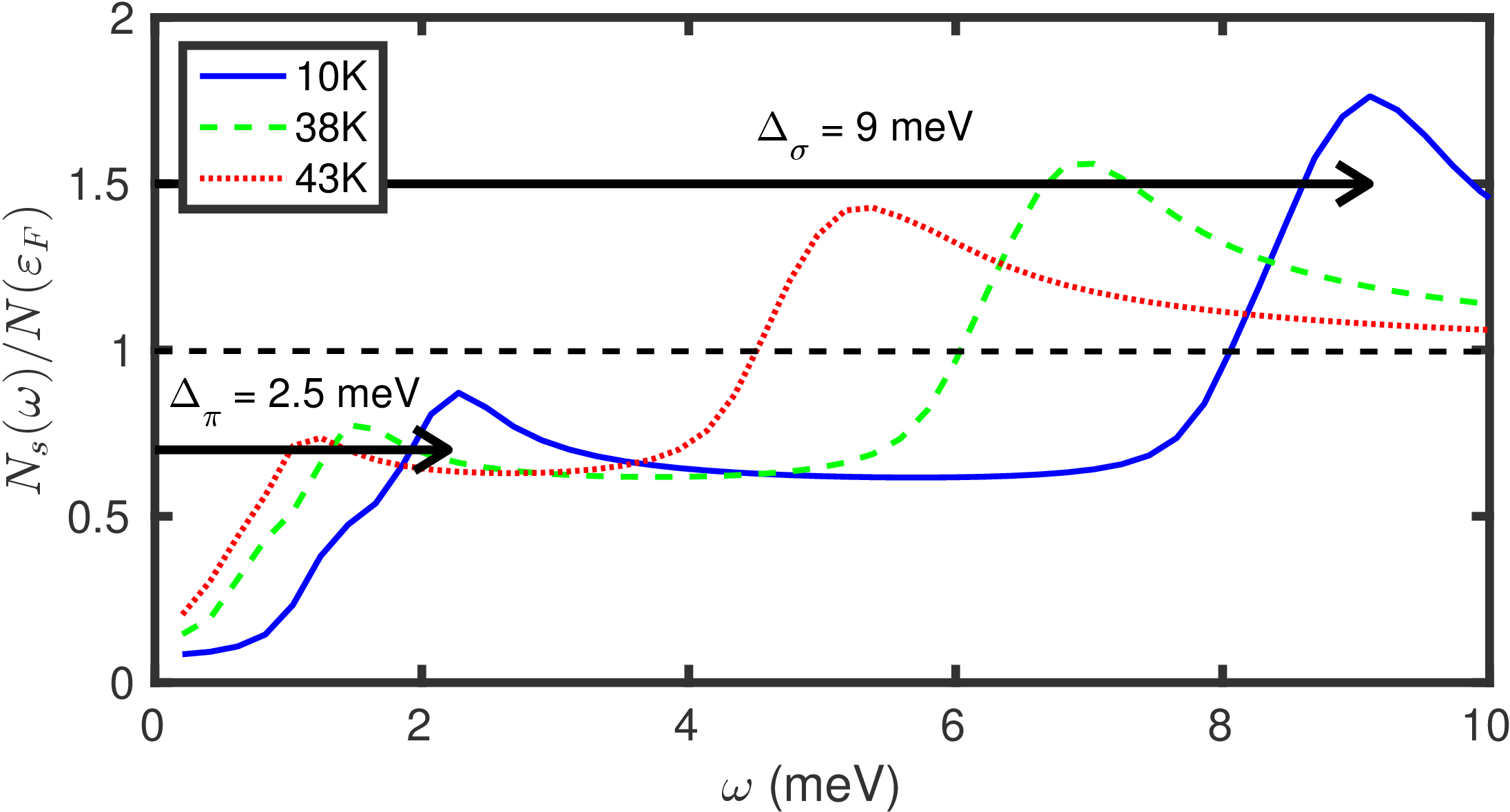
Figure 5: Quasiparticle DOS in the superconducting state for various temperatures [obtained using \(\Delta(\omega=0)\)]. The dashed black line is the normal state DOS taken from the top of Figure 1 and normalized to 1 at the Fermi level. The superconducting DOS \(N_{\rm S}(\omega)\) was scaled so that its high energy tail becomes 1 beyond the highest phonon energy. The two-gap nature of MgB₂ is clearly seen, and can be associated with the \(\sigma\) and \(\pi\) sheets on its Fermi surface, as shown in Figure 6 below.

• MgB2.imag_aniso_gap_FS_XX

  This file contains the superconducting gap on the Fermi surface. The first three columns contain the 3 Cartesian coordinates of each k-point, the 4th column is the band index within the chosen energy window, the 5th column is the energy difference with respect to the Fermi level. Only states within 0.2 eV of the Fermi energy are considered. The 6th column is the superconducting gap in eV. A 3D rendering of superconducting gap on top of the Fermi surface sheets is shown in Figure 6 below.

• MgB2.imag_aniso_gap_XX_YY.cube

  This file contains the same information as MgB2.imag_aniso_gap_FS_XX, in a format compatible with VESTA. This is suitable for mapping the gap on the Fermi surface. Here YY represents the band number within the chosen energy window during the EPW calculation.

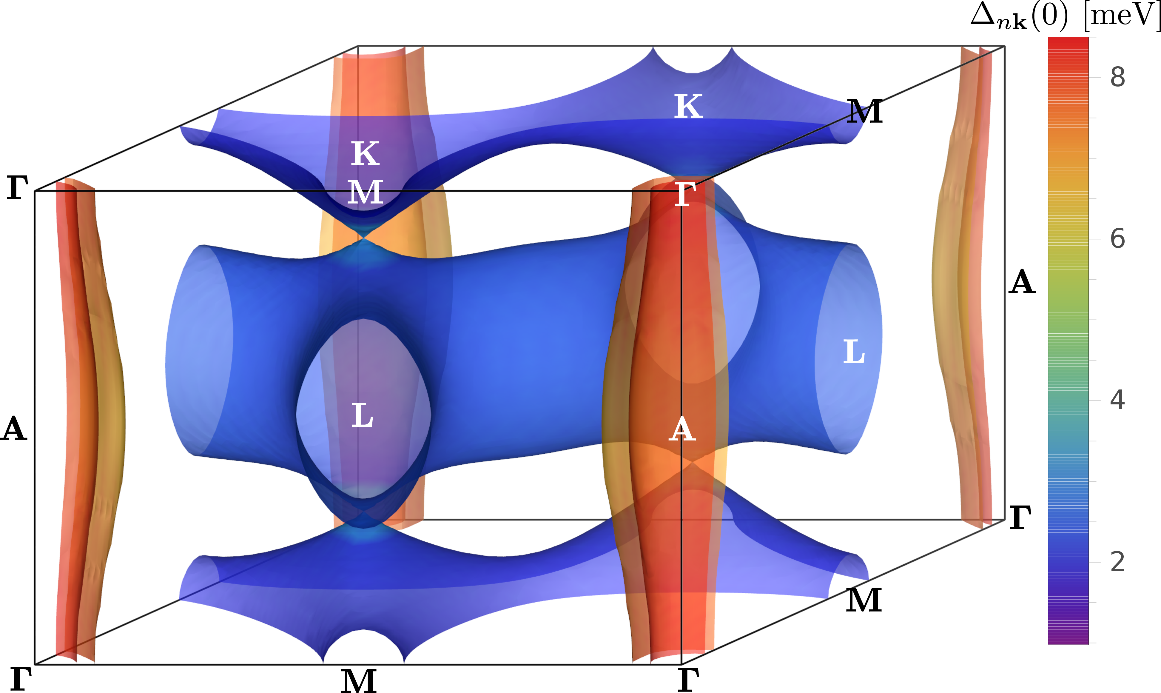
Figure 6: The superconducting energy gap of MgB₂, calculated at \(T=10`~K, mapped on the Fermi surface. The Fermi surface consists of two :math:\)sigma` sheets along the \(\Gamma-\Gamma\) lines, and two \(\pi\) sheets along the K-M and the H-L lines.

• MgB2.lambda_aniso

  This file contains 4 columns: KS eigenvalue \(E_{nk}\) relative to the Fermi level (eV), \(\lambda_{n{\bf k}}\), the wavevector \({\bf k}\), and the band index \(n\).

• MgB2.lambda_k_pairs

  This file contains the normalized distribution of the anisotropic electron-phonon coupling strength \(\lambda_{n{\bf k}}\) on the Fermi surface. This quantity is shown for example in Fig. 5b of Phys. Rev. B 87, 024505 (2013).

• MgB2.lambda_pairs

  This file contains the normalized distribution of the anisotropic electron-phonon coupling strength \(\lambda_{n{\bf k},n'{\bf k}'}\) on the Fermi surface.

• MgB2.fe_XX

  This file contains the free energy in the superconducting state.

• MgB2.lambda_FS

  This file contains \(\lambda_{n{\bf k}}\) on the Fermi surface. The first three columns represent Cartesian coordinates of the k-point, the 4th column is the band index within the specified energy window, the 5th column is the energy relative to the Fermi level. Only states within 0.2 eV of the Fermi energy are considered. The 6th column is \(\lambda_{n{\bf k}}\).

• MgB2.lambda_YY.cube

  This file contains the same information as MgB2.lambda_FS but can be read by VESTA for direct visualization. Note that YY is the band index within the specified energy window.

Note for expert users

If you wish to reproduce Figure 6 above (showing the map of the superconducting gap on the Fermi surface) you can use two python scripts from the following tar file

fermi.tar

The following video explains how to use the scripts in conjunction with VESTA to obtain Figure 6.

This video tutorial can also be found here.